Nano-Hexapod - Test Bench

Table of ContentsClose

1. Encoders fixed to the Struts - Dynamics
2. Encoders fixed to the plates - Dynamics
3. Decentralized High Authority Control with Integral Force Feedback
4. Functions

This report is also available as a pdf.

This document is dedicated to the experimental study of the nano-hexapod shown in Figure 1.

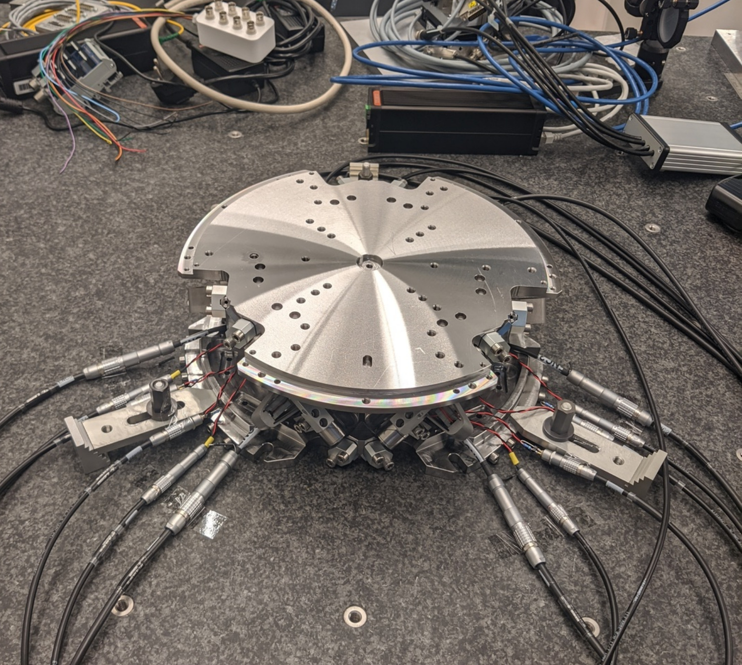
Figure 1: Nano-Hexapod

Note

Here are the documentation of the equipment used for this test bench (lots of them are shwon in Figure 2):

Voltage Amplifier: PiezoDrive PD200
Amplified Piezoelectric Actuator: Cedrat APA300ML
DAC/ADC: Speedgoat IO313
Encoder: Renishaw Vionic and used Ruler
Interferometers: Attocube

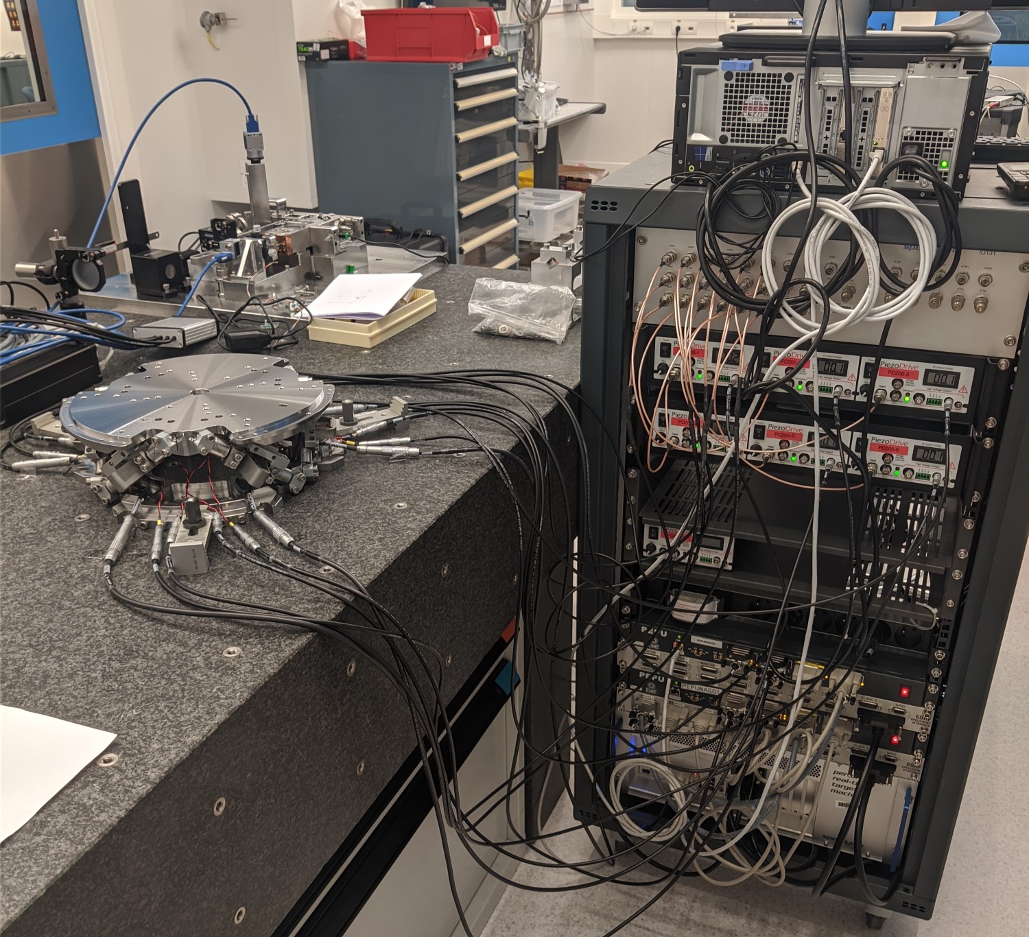
Figure 2: Nano-Hexapod and the control electronics

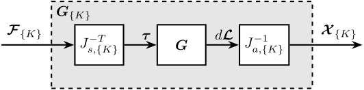
In Figure 3 is shown a block diagram of the experimental setup. When possible, the notations are consistent with this diagram and summarized in Table 1.

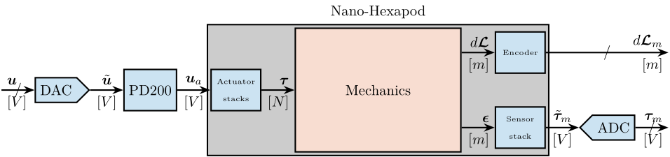
Figure 3: Block diagram of the system with named signals

Table 1: List of signals
	Unit	Matlab	Vector	Elements
Control Input (wanted DAC voltage)	`[V]`	`u`	$u$	$u_{i}$
DAC Output Voltage	`[V]`	`u`	$\tilde{u}$	${\tilde{u}}_{i}$
PD200 Output Voltage	`[V]`	`ua`	$u_{a}$	$u_{a, i}$
Actuator applied force	`[N]`	`tau`	$τ$	$τ_{i}$
Strut motion	`[m]`	`dL`	$d L$	$d L_{i}$
Encoder measured displacement	`[m]`	`dLm`	$d L_{m}$	$d L_{m, i}$
Force Sensor strain	`[m]`	`epsilon`	$ϵ$	$ϵ_{i}$
Force Sensor Generated Voltage	`[V]`	`taum`	${\tilde{τ}}_{m}$	${\tilde{τ}}_{m, i}$
Measured Generated Voltage	`[V]`	`taum`	$τ_{m}$	$τ_{m, i}$
Motion of the top platform	`[m,rad]`	`dX`	$d X$	$d X_{i}$
Metrology measured displacement	`[m,rad]`	`dXm`	$d X_{m}$	$d X_{m, i}$

This document is divided in the following sections:

Section 1: the dynamics of the nano-hexapod when the encoders are fixed to the struts is studied.
Section 2: the same is done when the encoders are fixed to the plates.
Section 3: a decentralized HAC-LAC strategy is studied and implemented.

1. Encoders fixed to the Struts - Dynamics

In this section, the encoders are fixed to the struts.

It is divided in the following sections:

Section 1.1: the transfer function matrix from the actuators to the force sensors and to the encoders is experimentally identified.
Section 1.2: the obtained FRF matrix is compared with the dynamics of the simscape model
Section 1.3: decentralized Integral Force Feedback (IFF) is applied and its performances are evaluated.
Section 1.4: a modal analysis of the nano-hexapod is performed

1.1. Identification of the dynamics

1.1.1. Load Measurement Data

Copy
%% Load Identification Data
meas_data_lf = {};

for i = 1:6
    meas_data_lf(i) = {load(sprintf('mat/frf_data_exc_strut_%i_noise_lf.mat', i), 't', 'Va', 'Vs', 'de')};
    meas_data_hf(i) = {load(sprintf('mat/frf_data_exc_strut_%i_noise_hf.mat', i), 't', 'Va', 'Vs', 'de')};
end

1.1.2. Spectral Analysis - Setup

Copy
%% Setup useful variables
% Sampling Time [s]
Ts = (meas_data_lf{1}.t(end) - (meas_data_lf{1}.t(1)))/(length(meas_data_lf{1}.t)-1);

% Sampling Frequency [Hz]
Fs = 1/Ts;

% Hannning Windows
win = hanning(ceil(1*Fs));

% And we get the frequency vector
[~, f] = tfestimate(meas_data_lf{1}.Va, meas_data_lf{1}.de, win, [], [], 1/Ts);

i_lf = f < 250; % Points for low frequency excitation
i_hf = f > 250; % Points for high frequency excitation

1.1.3. Transfer function from Actuator to Encoder

First, let’s compute the coherence from the excitation voltage and the displacement as measured by the encoders (Figure 4).

Copy
%% Coherence
coh_dvf = zeros(length(f), 6, 6);

for i = 1:6
    coh_dvf_lf = mscohere(meas_data_lf{i}.Va, meas_data_lf{i}.de, win, [], [], 1/Ts);
    coh_dvf_hf = mscohere(meas_data_hf{i}.Va, meas_data_hf{i}.de, win, [], [], 1/Ts);
    coh_dvf(:,:,i) = [coh_dvf_lf(i_lf, :); coh_dvf_hf(i_hf, :)];
end

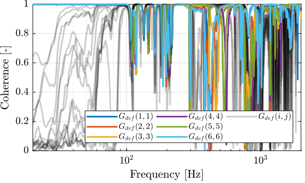
Figure 4: Obtained coherence for the DVF plant

Then the 6x6 transfer function matrix is estimated (Figure 5).

Copy
%% DVF Plant (transfer function from u to dLm)
G_dvf = zeros(length(f), 6, 6);

for i = 1:6
    G_dvf_lf = tfestimate(meas_data_lf{i}.Va, meas_data_lf{i}.de, win, [], [], 1/Ts);
    G_dvf_hf = tfestimate(meas_data_hf{i}.Va, meas_data_hf{i}.de, win, [], [], 1/Ts);
    G_dvf(:,:,i) = [G_dvf_lf(i_lf, :); G_dvf_hf(i_hf, :)];
end

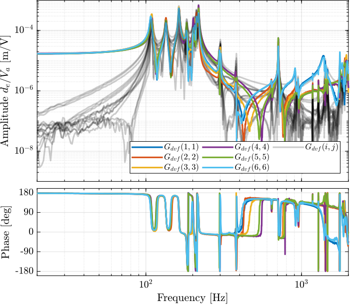
Figure 5: Measured FRF for the DVF plant

1.1.4. Transfer function from Actuator to Force Sensor

First, let’s compute the coherence from the excitation voltage and the displacement as measured by the encoders (Figure 6).

Copy
%% Coherence for the IFF plant
coh_iff = zeros(length(f), 6, 6);

for i = 1:6
    coh_iff_lf = mscohere(meas_data_lf{i}.Va, meas_data_lf{i}.Vs, win, [], [], 1/Ts);
    coh_iff_hf = mscohere(meas_data_hf{i}.Va, meas_data_hf{i}.Vs, win, [], [], 1/Ts);
    coh_iff(:,:,i) = [coh_iff_lf(i_lf, :); coh_iff_hf(i_hf, :)];
end

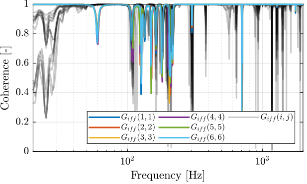
Figure 6: Obtained coherence for the IFF plant

Then the 6x6 transfer function matrix is estimated (Figure 7).

Copy
%% IFF Plant
G_iff = zeros(length(f), 6, 6);

for i = 1:6
    G_iff_lf = tfestimate(meas_data_lf{i}.Va, meas_data_lf{i}.Vs, win, [], [], 1/Ts);
    G_iff_hf = tfestimate(meas_data_hf{i}.Va, meas_data_hf{i}.Vs, win, [], [], 1/Ts);
    G_iff(:,:,i) = [G_iff_lf(i_lf, :); G_iff_hf(i_hf, :)];
end

Figure 7: Measured FRF for the IFF plant

1.1.5. Save Identified Plants

Copy
save('matlab/mat/identified_plants_enc_struts.mat', 'f', 'Ts', 'G_iff', 'G_dvf')

1.2. Comparison with the Simscape Model

In this section, the measured dynamics is compared with the dynamics estimated from the Simscape model.

1.2.1. Load measured FRF

Copy
%% Load data
load('identified_plants_enc_struts.mat', 'f', 'Ts', 'G_iff', 'G_dvf')

1.2.2. Dynamics from Actuator to Force Sensors

Copy
%% Initialize Nano-Hexapod
n_hexapod = initializeNanoHexapodFinal('flex_bot_type', '4dof', ...
                                       'flex_top_type', '4dof', ...
                                       'motion_sensor_type', 'struts', ...
                                       'actuator_type', '2dof');

Copy
%% Identify the IFF Plant (transfer function from u to taum)
clear io; io_i = 1;
io(io_i) = linio([mdl, '/du'],  1, 'openinput');   io_i = io_i + 1; % Actuator Inputs
io(io_i) = linio([mdl, '/dum'],  1, 'openoutput'); io_i = io_i + 1; % Force Sensors

Giff = exp(-s*Ts)*linearize(mdl, io, 0.0, options);

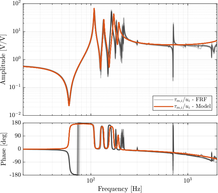
Figure 8: Diagonal elements of the IFF Plant

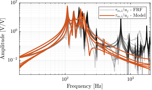
Figure 9: Off diagonal elements of the IFF Plant

1.2.3. Dynamics from Actuator to Encoder

Copy
%% Initialization of the Nano-Hexapod
n_hexapod = initializeNanoHexapodFinal('flex_bot_type', '4dof', ...
                                       'flex_top_type', '4dof', ...
                                       'motion_sensor_type', 'struts', ...
                                       'actuator_type', 'flexible');

Copy
%% Identify the DVF Plant (transfer function from u to dLm)
clear io; io_i = 1;
io(io_i) = linio([mdl, '/du'],  1, 'openinput');  io_i = io_i + 1; % Actuator Inputs
io(io_i) = linio([mdl, '/D'],  1, 'openoutput'); io_i = io_i + 1; % Encoders

Gdvf = exp(-s*Ts)*linearize(mdl, io, 0.0, options);

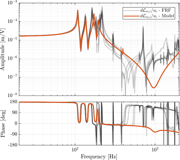
Figure 10: Diagonal elements of the DVF Plant

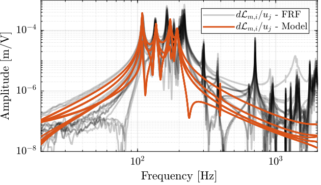
Figure 11: Off diagonal elements of the DVF Plant

1.2.4. Effect of a change in bending damping of the joints

Copy
%% Tested bending dampings [Nm/(rad/s)]
cRs = [1e-3, 5e-3, 1e-2, 5e-2, 1e-1];

Copy
%% Identify the DVF Plant (transfer function from u to dLm)
clear io; io_i = 1;
io(io_i) = linio([mdl, '/du'],  1, 'openinput');  io_i = io_i + 1; % Actuator Inputs
io(io_i) = linio([mdl, '/D'],  1, 'openoutput'); io_i = io_i + 1; % Encoders

Then the identification is performed for all the values of the bending damping.

Copy
%% Idenfity the transfer function from actuator to encoder for all bending dampins
Gs = {zeros(length(cRs), 1)};

for i = 1:length(cRs)
    n_hexapod = initializeNanoHexapodFinal('flex_bot_type', '4dof', ...
                                           'flex_top_type', '4dof', ...
                                           'motion_sensor_type', 'struts', ...
                                           'actuator_type', 'flexible', ...
                                           'flex_bot_cRx', cRs(i), ...
                                           'flex_bot_cRy', cRs(i), ...
                                           'flex_top_cRx', cRs(i), ...
                                           'flex_top_cRy', cRs(i));

    G = exp(-s*Ts)*linearize(mdl, io, 0.0, options);
    G.InputName  = {'Va1', 'Va2', 'Va3', 'Va4', 'Va5', 'Va6'};
    G.OutputName = {'dL1', 'dL2', 'dL3', 'dL4', 'dL5', 'dL6'};

    Gs(i) = {G};
end

Could be nice
Actual damping is very small

1.2.5. Effect of a change in damping factor of the APA

Copy
%% Tested bending dampings [Nm/(rad/s)]
xis = [1e-3, 5e-3, 1e-2, 5e-2, 1e-1];

Copy
%% Identify the DVF Plant (transfer function from u to dLm)
clear io; io_i = 1;
io(io_i) = linio([mdl, '/du'],  1, 'openinput');  io_i = io_i + 1; % Actuator Inputs
io(io_i) = linio([mdl, '/D'],  1, 'openoutput'); io_i = io_i + 1; % Encoders

Copy
%% Idenfity the transfer function from actuator to encoder for all bending dampins
Gs = {zeros(length(xis), 1)};

for i = 1:length(xis)
    n_hexapod = initializeNanoHexapodFinal('flex_bot_type', '4dof', ...
                                           'flex_top_type', '4dof', ...
                                           'motion_sensor_type', 'struts', ...
                                           'actuator_type', 'flexible', ...
                                           'actuator_xi', xis(i));

    G = exp(-s*Ts)*linearize(mdl, io, 0.0, options);
    G.InputName  = {'Va1', 'Va2', 'Va3', 'Va4', 'Va5', 'Va6'};
    G.OutputName = {'dL1', 'dL2', 'dL3', 'dL4', 'dL5', 'dL6'};

    Gs(i) = {G};
end

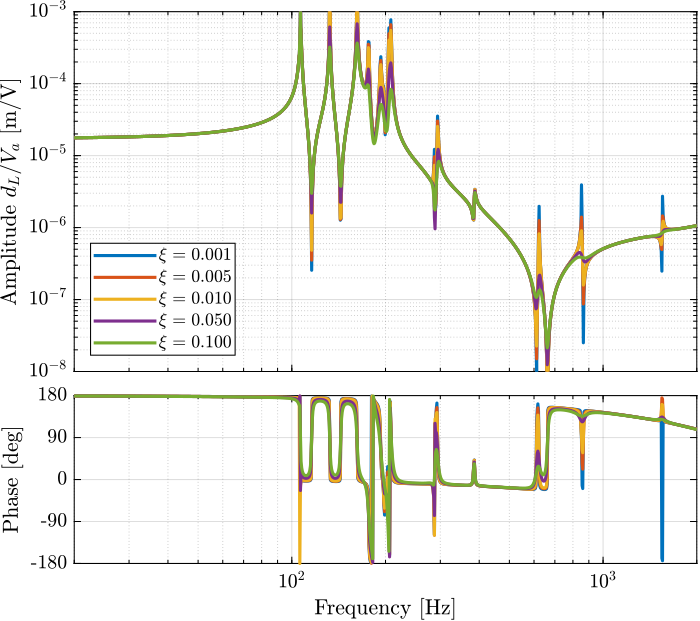
Figure 12: Effect of the APA damping factor $ξ$ on the dynamics from $u$ to $d L$

Important

Damping factor $ξ$ has a large impact on the damping of the “spurious resonances” at 200Hz and 300Hz.

Question

Why is the damping factor does not change the damping of the first peak?

1.2.6. Effect of a change in stiffness damping coef of the APA

Copym_coef = 1e1;

Copy
%% Tested bending dampings [Nm/(rad/s)]
k_coefs = [1e-6, 5e-6, 1e-5, 5e-5, 1e-4];

Copy
%% Identify the DVF Plant (transfer function from u to dLm)
clear io; io_i = 1;
io(io_i) = linio([mdl, '/du'],  1, 'openinput');  io_i = io_i + 1; % Actuator Inputs
io(io_i) = linio([mdl, '/D'],  1, 'openoutput'); io_i = io_i + 1; % Encoders

Copy
%% Idenfity the transfer function from actuator to encoder for all bending dampins
Gs = {zeros(length(k_coefs), 1)};
n_hexapod = initializeNanoHexapodFinal('flex_bot_type', '4dof', ...
                                       'flex_top_type', '4dof', ...
                                       'motion_sensor_type', 'struts', ...
                                       'actuator_type', 'flexible');

for i = 1:length(k_coefs)
    k_coef = k_coefs(i);

    G = exp(-s*Ts)*linearize(mdl, io, 0.0, options);
    G.InputName  = {'Va1', 'Va2', 'Va3', 'Va4', 'Va5', 'Va6'};
    G.OutputName = {'dL1', 'dL2', 'dL3', 'dL4', 'dL5', 'dL6'};

    Gs(i) = {G};
end

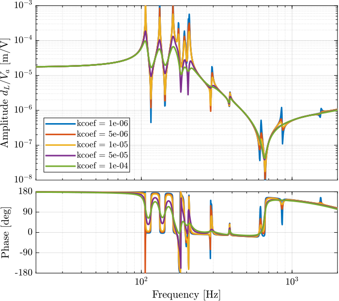
Figure 13: Effect of a change of the damping “stiffness coeficient” on the transfer function from $u$ to $d L$

1.2.7. Effect of a change in mass damping coef of the APA

Copy
k_coef = 1e-6;

Copy
%% Tested bending dampings [Nm/(rad/s)]
m_coefs = [1e1, 5e1, 1e2, 5e2, 1e3];

Copy
%% Identify the DVF Plant (transfer function from u to dLm)
clear io; io_i = 1;
io(io_i) = linio([mdl, '/du'],  1, 'openinput');  io_i = io_i + 1; % Actuator Inputs
io(io_i) = linio([mdl, '/D'],  1, 'openoutput'); io_i = io_i + 1; % Encoders

Copy
%% Idenfity the transfer function from actuator to encoder for all bending dampins
Gs = {zeros(length(m_coefs), 1)};
n_hexapod = initializeNanoHexapodFinal('flex_bot_type', '4dof', ...
                                       'flex_top_type', '4dof', ...
                                       'motion_sensor_type', 'struts', ...
                                       'actuator_type', 'flexible');

for i = 1:length(m_coefs)
    m_coef = m_coefs(i);

    G = exp(-s*Ts)*linearize(mdl, io, 0.0, options);
    G.InputName  = {'Va1', 'Va2', 'Va3', 'Va4', 'Va5', 'Va6'};
    G.OutputName = {'dL1', 'dL2', 'dL3', 'dL4', 'dL5', 'dL6'};

    Gs(i) = {G};
end

Figure 14: Effect of a change of the damping “mass coeficient” on the transfer function from $u$ to $d L$

1.2.8. Using Flexible model

Copy
d_aligns = [[-0.05,  -0.3,  0];
            [ 0,      0.5,  0];
            [-0.1,   -0.3,  0];
            [ 0,      0.3,  0];
            [-0.05,   0.05, 0];
            [0,       0,    0]]*1e-3;

Copyd_aligns = zeros(6,3);
% d_aligns(1,:) = [-0.05,  -0.3,  0]*1e-3;
d_aligns(2,:) = [ 0,      0.3,  0]*1e-3;

Copy
%% Initialize Nano-Hexapod
n_hexapod = initializeNanoHexapodFinal('flex_bot_type', '4dof', ...
                                       'flex_top_type', '4dof', ...
                                       'motion_sensor_type', 'struts', ...
                                       'actuator_type', 'flexible', ...
                                       'actuator_d_align', d_aligns);

Question

Why do we have smaller resonances when using flexible APA? On the test bench we have the same resonance as the 2DoF model. Could it be due to the compliance in other dof of the flexible model?

Copy
%% Identify the DVF Plant (transfer function from u to dLm)
clear io; io_i = 1;
io(io_i) = linio([mdl, '/du'],  1, 'openinput');  io_i = io_i + 1; % Actuator Inputs
io(io_i) = linio([mdl, '/D'],  1, 'openoutput'); io_i = io_i + 1; % Encoders

Gdvf = exp(-s*Ts)*linearize(mdl, io, 0.0, options);

Copy
%% Identify the IFF Plant (transfer function from u to taum)
clear io; io_i = 1;
io(io_i) = linio([mdl, '/du'],  1, 'openinput');   io_i = io_i + 1; % Actuator Inputs
io(io_i) = linio([mdl, '/dum'],  1, 'openoutput'); io_i = io_i + 1; % Force Sensors

Giff = exp(-s*Ts)*linearize(mdl, io, 0.0, options);

1.2.9. Flexible model + encoders fixed to the plates

Copy
%% Identify the IFF Plant (transfer function from u to taum)
clear io; io_i = 1;
io(io_i) = linio([mdl, '/du'],  1, 'openinput');   io_i = io_i + 1; % Actuator Inputs
io(io_i) = linio([mdl, '/D'],  1, 'openoutput'); io_i = io_i + 1; % Force Sensors

Copy
d_aligns = [[-0.05,  -0.3,  0];
            [ 0,      0.5,  0];
            [-0.1,   -0.3,  0];
            [ 0,      0.3,  0];
            [-0.05,   0.05, 0];
            [0,       0,    0]]*1e-3;

Copy
%% Initialize Nano-Hexapod
n_hexapod = initializeNanoHexapodFinal('flex_bot_type', '4dof', ...
                                       'flex_top_type', '4dof', ...
                                       'motion_sensor_type', 'struts', ...
                                       'actuator_type', 'flexible', ...
                                       'actuator_d_align', d_aligns);

Copy
Gdvf_struts = exp(-s*Ts)*linearize(mdl, io, 0.0, options);

Copy
%% Initialize Nano-Hexapod
n_hexapod = initializeNanoHexapodFinal('flex_bot_type', '4dof', ...
                                       'flex_top_type', '4dof', ...
                                       'motion_sensor_type', 'plates', ...
                                       'actuator_type', 'flexible', ...
                                       'actuator_d_align', d_aligns);

Copy
Gdvf_plates = exp(-s*Ts)*linearize(mdl, io, 0.0, options);

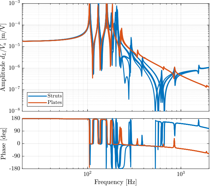
Figure 15: Comparison of the dynamics from $V_{a}$ to $d_{L}$ when the encoders are fixed to the struts (blue) and to the plates (red). APA are modeled as a flexible element.

1.3. Integral Force Feedback

In this section, the Integral Force Feedback (IFF) control strategy is applied to the nano-hexapod. The main goal of this to add damping to the nano-hexapod’s modes.

The control architecture is shown in Figure 16 where $K_{IFF}$ is a diagonal $6 \times 6$ controller.

The system as then a new input $u^{'}$ , and the transfer function from $u^{'}$ to $d L_{m}$ should be easier to control than the initial transfer function from $u$ to $d L_{m}$ .

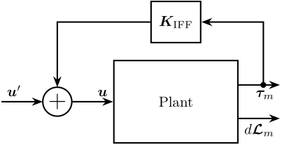
Figure 16: Integral Force Feedback Strategy

This section is structured as follow:

Section 1.3.1: Using the Simscape model (APA taken as 2DoF model), the transfer function from $u$ to $τ_{m}$ is identified. Based on the obtained dynamics, the control law is developed and the optimal gain is estimated using the Root Locus.
Section 1.3.2: Still using the Simscape model, the effect of the IFF gain on the the transfer function from $u^{'}$ to $d L_{m}$ is studied.
Section 1.3.3: The same is performed experimentally: several IFF gains are used and the damped plant is identified each time.
Section 1.3.4: The damped model and the identified damped system are compared for the optimal IFF gain. It is found that IFF indeed adds a lot of damping into the system. However it is not efficient in damping the spurious struts modes.
Section 1.3.5: Finally, a “flexible” model of the APA is used in the Simscape model and the optimally damped model is compared with the measurements.

1.3.1. IFF Control Law and Optimal Gain

Let’s use a model of the Nano-Hexapod with the encoders fixed to the struts and the APA taken as 2DoF model.

Copy
%% Initialize Nano-Hexapod
n_hexapod = initializeNanoHexapodFinal('flex_bot_type', '4dof', ...
                                       'flex_top_type', '4dof', ...
                                       'motion_sensor_type', 'struts', ...
                                       'actuator_type', '2dof');

The transfer function from $u$ to $τ_{m}$ is identified.

Copy
%% Identify the IFF Plant (transfer function from u to taum)
clear io; io_i = 1;
io(io_i) = linio([mdl, '/du'],  1, 'openinput');   io_i = io_i + 1; % Actuator Inputs
io(io_i) = linio([mdl, '/dum'],  1, 'openoutput'); io_i = io_i + 1; % Force Sensors

Giff = exp(-s*Ts)*linearize(mdl, io, 0.0, options);

The IFF controller is defined as shown below:

Copy
%% IFF Controller
Kiff_g1 = -(1/(s + 2*pi*40))*...    % LPF: provides integral action above 40Hz
           (s/(s + 2*pi*30))*...    % HPF: limit low frequency gain
           (1/(1 + s/2/pi/500))*... % LPF: more robust to high frequency resonances
           eye(6);                  % Diagonal 6x6 controller

Then, the poles of the system are shown in the complex plane as a function of the controller gain (i.e. Root Locus plot) in Figure 17. A gain of $400$ is chosen as the “optimal” gain as it visually seems to be the gain that adds the maximum damping to all the suspension modes simultaneously.

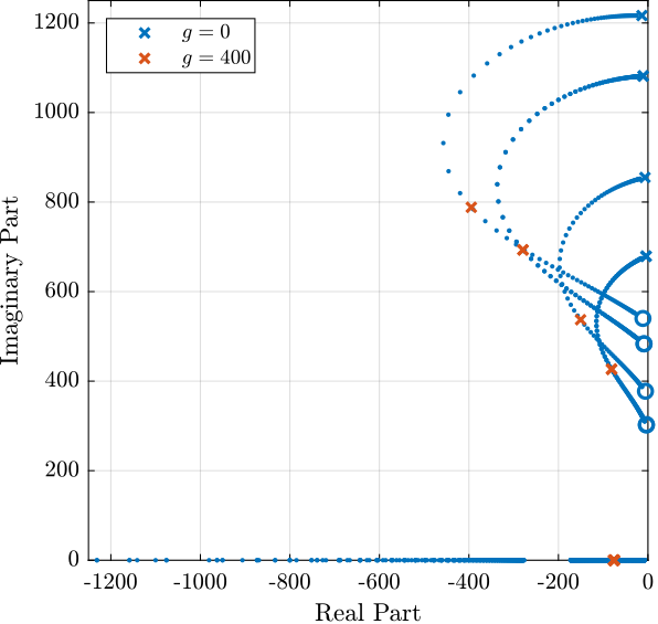
Figure 17: Root Locus for the IFF control strategy

Then the “optimal” IFF controller is:

Copy
%% IFF controller with Optimal gain
Kiff = 400*Kiff_g1;

And it is saved for further use.

Copy
save('mat/Kiff.mat', 'Kiff')

The bode plots of the “diagonal” elements of the loop gain are shown in Figure 18. It is shown that the phase and gain margins are quite high and the loop gain is large arround the resonances.

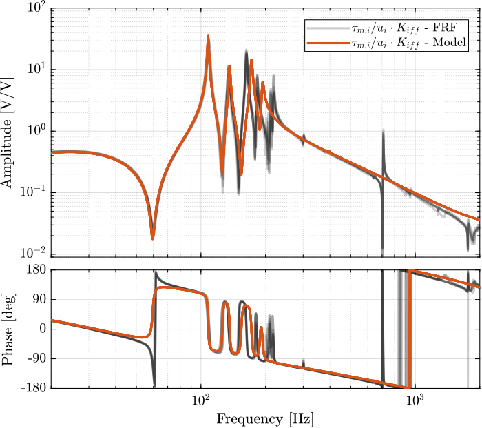
Figure 18: Bode plot of the “decentralized loop gain” $G_{iff} (i, i) \times K_{iff} (i, i)$

1.3.2. Effect of IFF on the plant - Simulations

Still using the Simscape model with encoders fixed to the struts and 2DoF APA, the IFF strategy is tested.

Copy
%% Initialize the Simscape model in closed loop
n_hexapod = initializeNanoHexapodFinal('flex_bot_type', '4dof', ...
                                       'flex_top_type', '4dof', ...
                                       'motion_sensor_type', 'struts', ...
                                       'actuator_type', '2dof', ...
                                       'controller_type', 'iff');

The following IFF gains are tried:

Copy
%% Tested IFF gains
iff_gains = [4, 10, 20, 40, 100, 200, 400];

And the transfer functions from $u^{'}$ to $d L_{m}$ are identified for all the IFF gains.

Copy
%% Identify the (damped) transfer function from u to dLm for different values of the IFF gain
Gd_iff = {zeros(1, length(iff_gains))};

clear io; io_i = 1;
io(io_i) = linio([mdl, '/du'], 1, 'openinput');  io_i = io_i + 1; % Actuator Inputs
io(io_i) = linio([mdl, '/dL'], 1, 'openoutput'); io_i = io_i + 1; % Strut Displacement (encoder)

for i = 1:length(iff_gains)
    Kiff = iff_gains(i)*Kiff_g1*eye(6); % IFF Controller
    Gd_iff(i) = {exp(-s*Ts)*linearize(mdl, io, 0.0, options)};

    isstable(Gd_iff{i})
end

The obtained dynamics are shown in Figure 19.

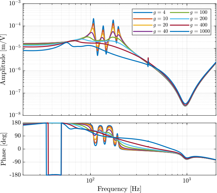
Figure 19: Effect of the IFF gain $g$ on the transfer function from $τ$ to $d L_{m}$

1.3.3. Effect of IFF on the plant - Experimental Results

The IFF strategy is applied experimentally and the transfer function from $u^{'}$ to $d L_{m}$ is identified for all the defined values of the gain.

1.3.3.1. Load Data

First load the identification data.

Copy
%% Load Identification Data
meas_iff_gains = {};

for i = 1:length(iff_gains)
    meas_iff_gains(i) = {load(sprintf('mat/iff_strut_1_noise_g_%i.mat', iff_gains(i)), 't', 'Vexc', 'Vs', 'de', 'u')};
end

1.3.3.2. Spectral Analysis - Setup

And define the useful variables that will be used for the identification using the tfestimate function.

Copy
%% Setup useful variables
% Sampling Time [s]
Ts = (meas_iff_gains{1}.t(end) - (meas_iff_gains{1}.t(1)))/(length(meas_iff_gains{1}.t)-1);

% Sampling Frequency [Hz]
Fs = 1/Ts;

% Hannning Windows
win = hanning(ceil(1*Fs));

% And we get the frequency vector
[~, f] = tfestimate(meas_iff_gains{1}.Vexc, meas_iff_gains{1}.de, win, [], [], 1/Ts);

1.3.3.3. DVF Plant

The transfer functions are estimated for all the values of the gain.

Copy
%% DVF Plant (transfer function from u to dLm)
G_iff_gains = {};

for i = 1:length(iff_gains)
    G_iff_gains{i} = tfestimate(meas_iff_gains{i}.Vexc, meas_iff_gains{i}.de(:,1), win, [], [], 1/Ts);
end

The obtained dynamics as shown in the bode plot in Figure 20. The dashed curves are the results obtained using the model, and the solid curves the results from the experimental identification.

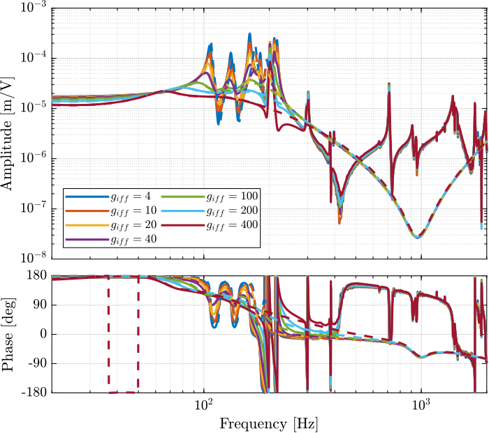
Figure 20: Transfer function from $u$ to $d L_{m}$ for multiple values of the IFF gain

The bode plot is then zoomed on the suspension modes of the nano-hexapod in Figure 21.

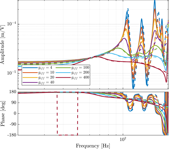
Figure 21: Transfer function from $u$ to $d L_{m}$ for multiple values of the IFF gain (Zoom)

Important

The IFF control strategy is very effective for the damping of the suspension modes. It however does not damp the modes at 200Hz, 300Hz and 400Hz (flexible modes of the APA).

Also, the experimental results and the models obtained from the Simscape model are in agreement concerning the damped system (up to the flexible modes).

1.3.3.4. Experimental Results - Comparison of the un-damped and fully damped system

The un-damped and damped experimental plants are compared in Figure 22 (diagonal terms).

It is very clear that all the suspension modes are very well damped thanks to IFF. However, there is little to no effect on the flexible modes of the struts and of the plate.

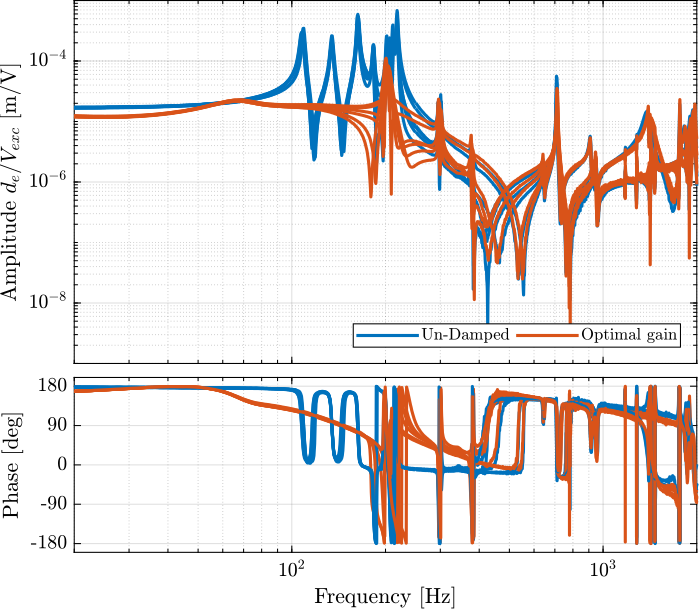
Figure 22: Comparison of the diagonal elements of the tranfer function from $u$ to $d L_{m}$ without active damping and with optimal IFF gain

1.3.4. Experimental Results - Damped Plant with Optimal gain

Let’s now look at the $6 \times 6$ damped plant with the optimal gain $g = 400$ .

1.3.4.1. Load Data

The experimental data are loaded.

Copy
%% Load Identification Data
meas_iff_struts = {};

for i = 1:6
    meas_iff_struts(i) = {load(sprintf('mat/iff_strut_%i_noise_g_400.mat', i), 't', 'Vexc', 'Vs', 'de', 'u')};
end

1.3.4.2. Spectral Analysis - Setup

And the parameters useful for the spectral analysis are defined.

Copy
%% Setup useful variables
% Sampling Time [s]
Ts = (meas_iff_struts{1}.t(end) - (meas_iff_struts{1}.t(1)))/(length(meas_iff_struts{1}.t)-1);

% Sampling Frequency [Hz]
Fs = 1/Ts;

% Hannning Windows
win = hanning(ceil(1*Fs));

% And we get the frequency vector
[~, f] = tfestimate(meas_iff_struts{1}.Vexc, meas_iff_struts{1}.de, win, [], [], 1/Ts);

1.3.4.3. DVF Plant

Finally, the $6 \times 6$ plant is identified using the tfestimate function.

Copy
%% DVF Plant (transfer function from u to dLm)
G_iff_opt = {};

for i = 1:6
    G_iff_opt{i} = tfestimate(meas_iff_struts{i}.Vexc, meas_iff_struts{i}.de, win, [], [], 1/Ts);
end

The obtained diagonal elements are compared with the model in Figure 23.

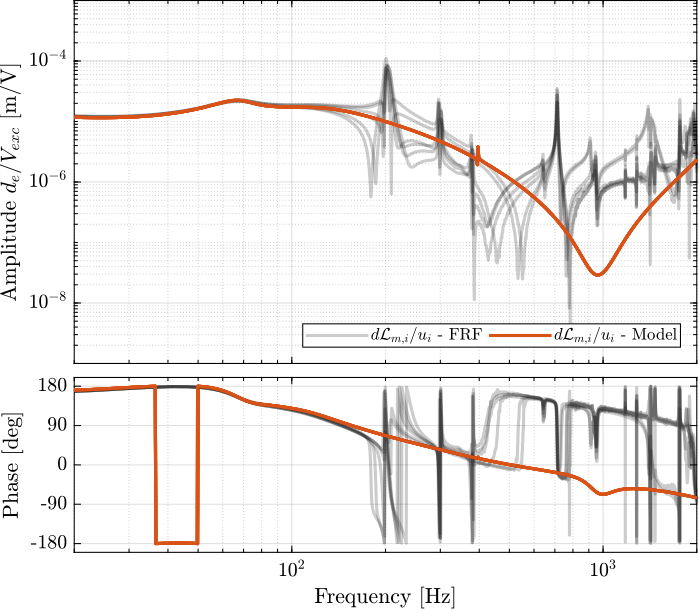
Figure 23: Comparison of the diagonal elements of the transfer functions from $u$ to $d L_{m}$ with active damping (IFF) applied with an optimal gain $g = 400$

And all the off-diagonal elements are compared with the model in Figure 24.

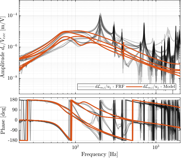
Figure 24: Comparison of the off-diagonal elements of the transfer functions from $u$ to $d L_{m}$ with active damping (IFF) applied with an optimal gain $g = 400$

Important

With the IFF control strategy applied and the optimal gain used, the suspension modes are very well damped. Remains the un-damped flexible modes of the APA (200Hz, 300Hz, 400Hz), and the modes of the plates (700Hz).

The Simscape model and the experimental results are in very good agreement.

1.3.5. Comparison with the Flexible model

When using the 2-DoF model for the APA, the flexible modes of the struts were not modelled, and it was the main limitation of the model. Now, let’s use a flexible model for the APA, and see if the obtained damped plant using the model is similar to the measured dynamics.

First, the nano-hexapod is initialized.

Copy
%% Estimated misalignement of the struts
d_aligns = [[-0.05,  -0.3,  0];
            [ 0,      0.5,  0];
            [-0.1,   -0.3,  0];
            [ 0,      0.3,  0];
            [-0.05,   0.05, 0];
            [0,       0,    0]]*1e-3;


%% Initialize Nano-Hexapod
n_hexapod = initializeNanoHexapodFinal('flex_bot_type', '4dof', ...
                                       'flex_top_type', '4dof', ...
                                       'motion_sensor_type', 'struts', ...
                                       'actuator_type', 'flexible', ...
                                       'actuator_d_align', d_aligns, ...
                                       'controller_type', 'iff');

And the “optimal” controller is loaded.

Copy
%% Optimal IFF controller
load('Kiff.mat', 'Kiff');

The transfer function from $u^{'}$ to $d L_{m}$ is identified using the Simscape model.

Copy
%% Linearized inputs/outputs
clear io; io_i = 1;
io(io_i) = linio([mdl, '/du'],  1, 'openinput');  io_i = io_i + 1; % Actuator Inputs
io(io_i) = linio([mdl, '/dL'],  1, 'openoutput'); io_i = io_i + 1; % Strut Displacement (encoder)

%% Identification of the plant
Gd_iff = exp(-s*Ts)*linearize(mdl, io, 0.0, options);

The obtained diagonal elements are shown in Figure 25 while the off-diagonal elements are shown in Figure 26.

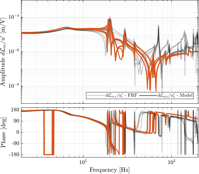
Figure 25: Diagonal elements of the transfer function from $u^{'}$ to $d L_{m}$ - comparison of the measured FRF and the identified dynamics using the flexible model

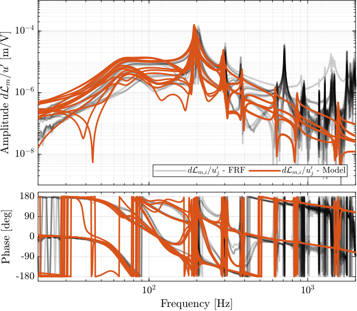
Figure 26: Off-diagonal elements of the transfer function from $u^{'}$ to $d L_{m}$ - comparison of the measured FRF and the identified dynamics using the flexible model

Important

Using flexible models for the APA, the agreement between the Simscape model of the nano-hexapod and the measured FRF is very good.

Only the flexible mode of the top-plate is not appearing in the model which is very logical as the top plate is taken as a solid body.

1.3.6. Conclusion

Important

The decentralized Integral Force Feedback strategy applied on the nano-hexapod is very effective in damping all the suspension modes.

The Simscape model (especially when using a flexible model for the APA) is shown to be very accurate, even when IFF is applied.

1.4. Modal Analysis

Several 3-axis accelerometers are fixed on the top platform of the nano-hexapod as shown in Figure 31.

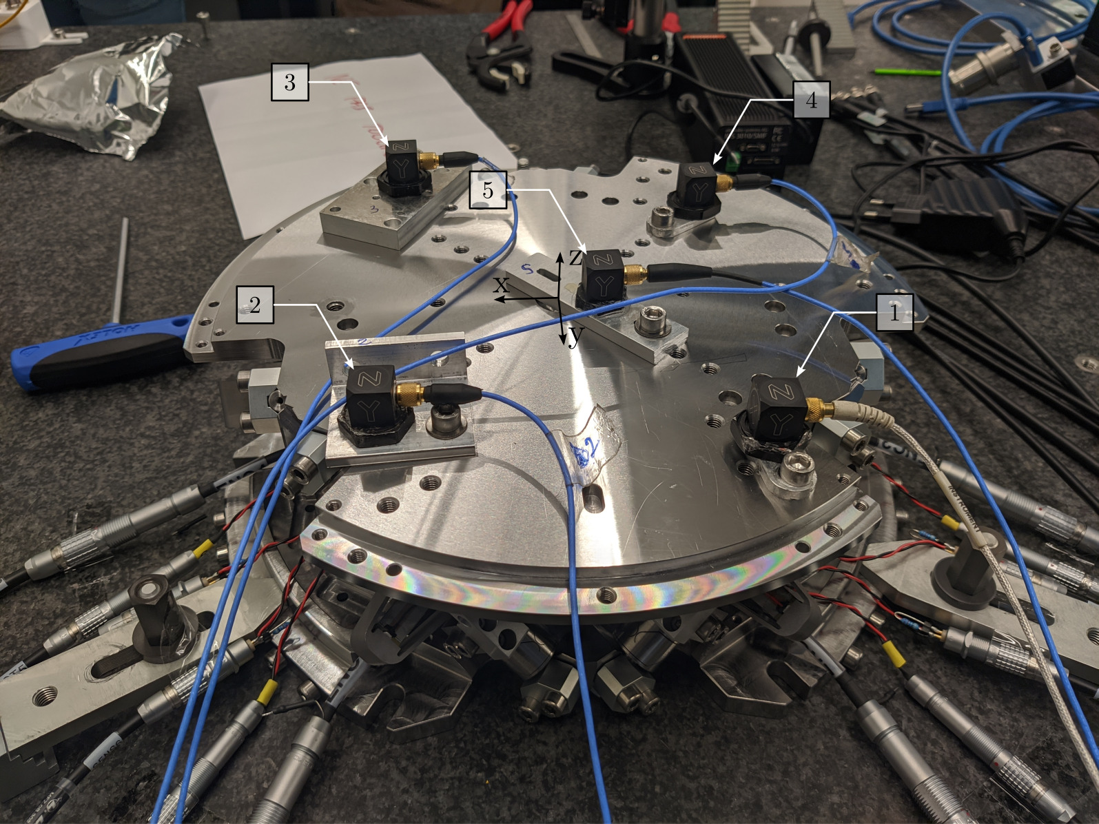
Figure 27: Location of the accelerometers on top of the nano-hexapod

The top platform is then excited using an instrumented hammer as shown in Figure 28.

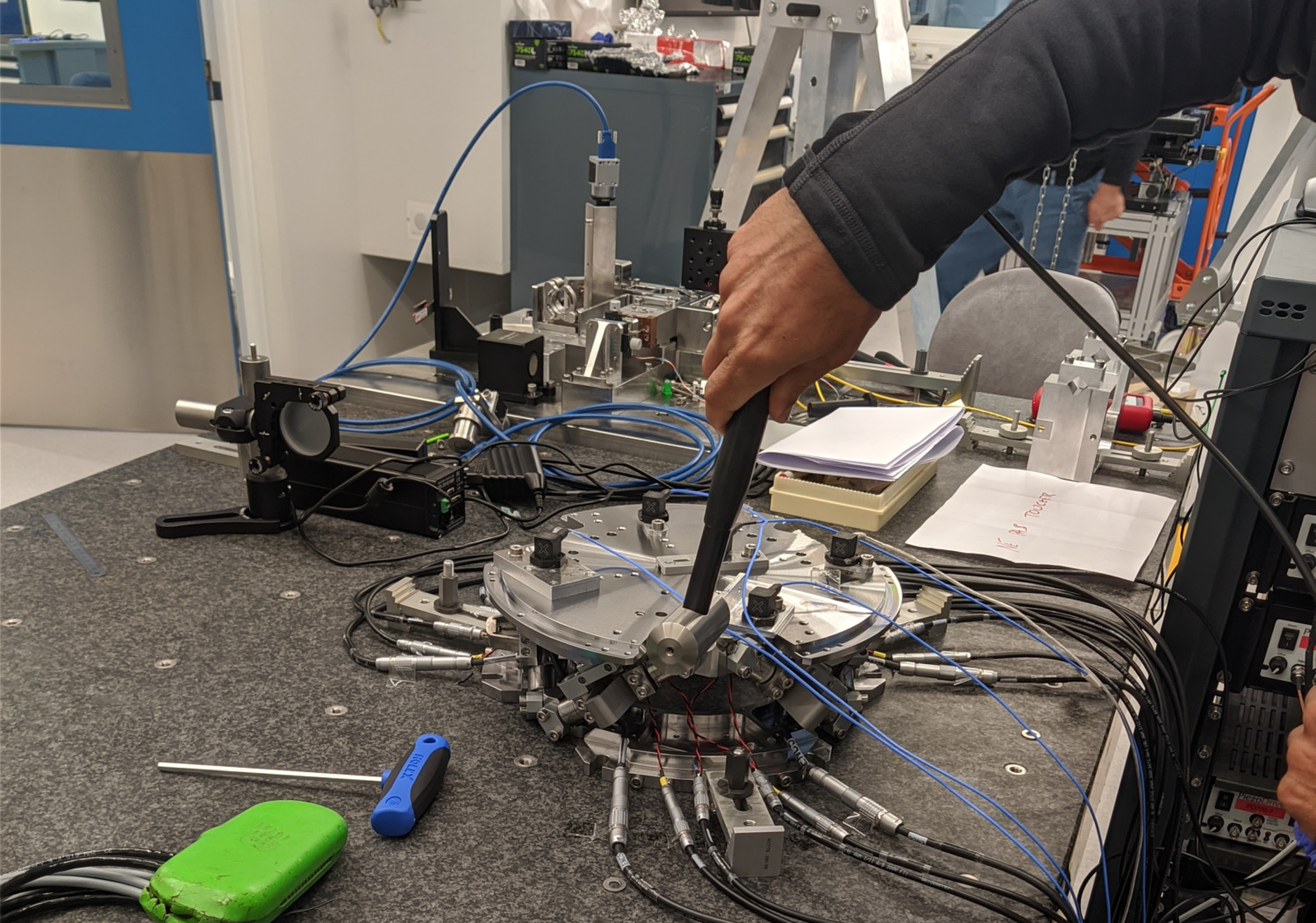
Figure 28: Example of an excitation using an instrumented hammer

From this experiment, the resonance frequencies and the associated mode shapes can be computed (Section 1.4.1). Then, in Section 1.4.2, the vertical compliance of the nano-hexapod is experimentally estimated. Finally, in Section 1.4.3, the measured compliance is compare with the estimated one from the Simscape model.

1.4.1. Obtained Mode Shapes

We can observe the mode shapes of the first 6 modes that are the suspension modes (the plate is behaving as a solid body) in Figure 29.

Figure 29: Measured mode shapes for the first six modes

Then, there is a mode at 692Hz which corresponds to a flexible mode of the top plate (Figure 30).

Figure 30: First flexible mode at 692Hz

The obtained modes are summarized in Table 2.

Table 2: Description of the identified modes
Mode	Freq. [Hz]	Description
1	105	Suspension Mode: Y-translation
2	107	Suspension Mode: X-translation
3	131	Suspension Mode: Z-translation
4	161	Suspension Mode: Y-tilt
5	162	Suspension Mode: X-tilt
6	180	Suspension Mode: Z-rotation
7	692	(flexible) Membrane mode of the top platform

1.4.2. Nano-Hexapod Compliance - Effect of IFF

In this section, we wish to estimated the effectiveness of the IFF strategy concerning the compliance.

The top plate is excited vertically using the instrumented hammer two times:

no control loop is used
decentralized IFF is used

The data is loaded.

Copy
frf_ol  = load('Measurement_Z_axis.mat'); % Open-Loop
frf_iff = load('Measurement_Z_axis_damped.mat'); % IFF

The mean vertical motion of the top platform is computed by averaging all 5 accelerometers.

Copy
%% Multiply by 10 (gain in m/s^2/V) and divide by 5 (number of accelerometers)
d_frf_ol = 10/5*(frf_ol.FFT1_H1_4_1_RMS_Y_Mod + frf_ol.FFT1_H1_7_1_RMS_Y_Mod + frf_ol.FFT1_H1_10_1_RMS_Y_Mod + frf_ol.FFT1_H1_13_1_RMS_Y_Mod + frf_ol.FFT1_H1_16_1_RMS_Y_Mod)./(2*pi*frf_ol.FFT1_H1_16_1_RMS_X_Val).^2;
d_frf_iff = 10/5*(frf_iff.FFT1_H1_4_1_RMS_Y_Mod + frf_iff.FFT1_H1_7_1_RMS_Y_Mod + frf_iff.FFT1_H1_10_1_RMS_Y_Mod + frf_iff.FFT1_H1_13_1_RMS_Y_Mod + frf_iff.FFT1_H1_16_1_RMS_Y_Mod)./(2*pi*frf_iff.FFT1_H1_16_1_RMS_X_Val).^2;

The vertical compliance (magnitude of the transfer function from a vertical force applied on the top plate to the vertical motion of the top plate) is shown in Figure 31.

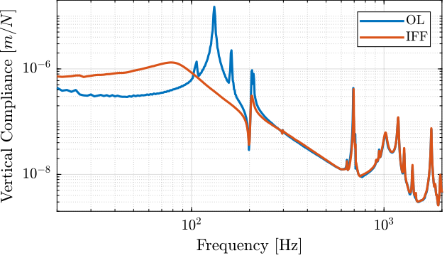
Figure 31: Measured vertical compliance with and without IFF

Important

From Figure 31, it is clear that the IFF control strategy is very effective in damping the suspensions modes of the nano-hexapod. It also has the effect of (slightly) degrading the vertical compliance at low frequency.

It also seems some damping can be added to the modes at around 205Hz which are flexible modes of the struts.

1.4.3. Comparison with the Simscape Model

Let’s now compare the measured vertical compliance with the vertical compliance as estimated from the Simscape model.

The transfer function from a vertical external force to the absolute motion of the top platform is identified (with and without IFF) using the Simscape model. The comparison is done in Figure 32. Again, the model is quite accurate!

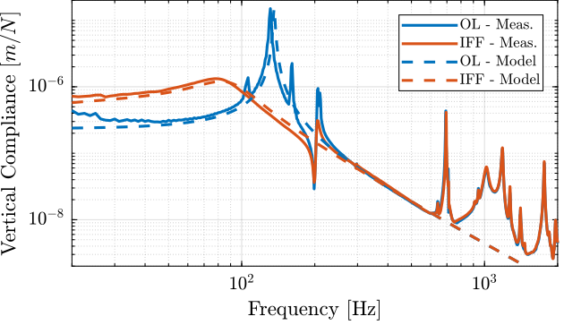
Figure 32: Measured vertical compliance with and without IFF

1.5. Conclusion

Important

From the previous analysis, several conclusions can be drawn:

Decentralized IFF is very effective in damping the “suspension” modes of the nano-hexapod (Figure 22)
Decentralized IFF does not damp the “spurious” modes of the struts nor the flexible modes of the top plate (Figure 22)
Even though the Simscape model and the experimentally measured FRF are in good agreement (Figures 25 and 26), the obtain dynamics from the control inputs $u$ and the encoders $d L_{m}$ is very difficult to control

Therefore, in the following sections, the encoders will be fixed to the plates. The goal is to be less sensitive to the flexible modes of the struts.

2. Encoders fixed to the plates - Dynamics

In this section, the encoders are fixed to the plates rather than to the struts as shown in Figure 33.

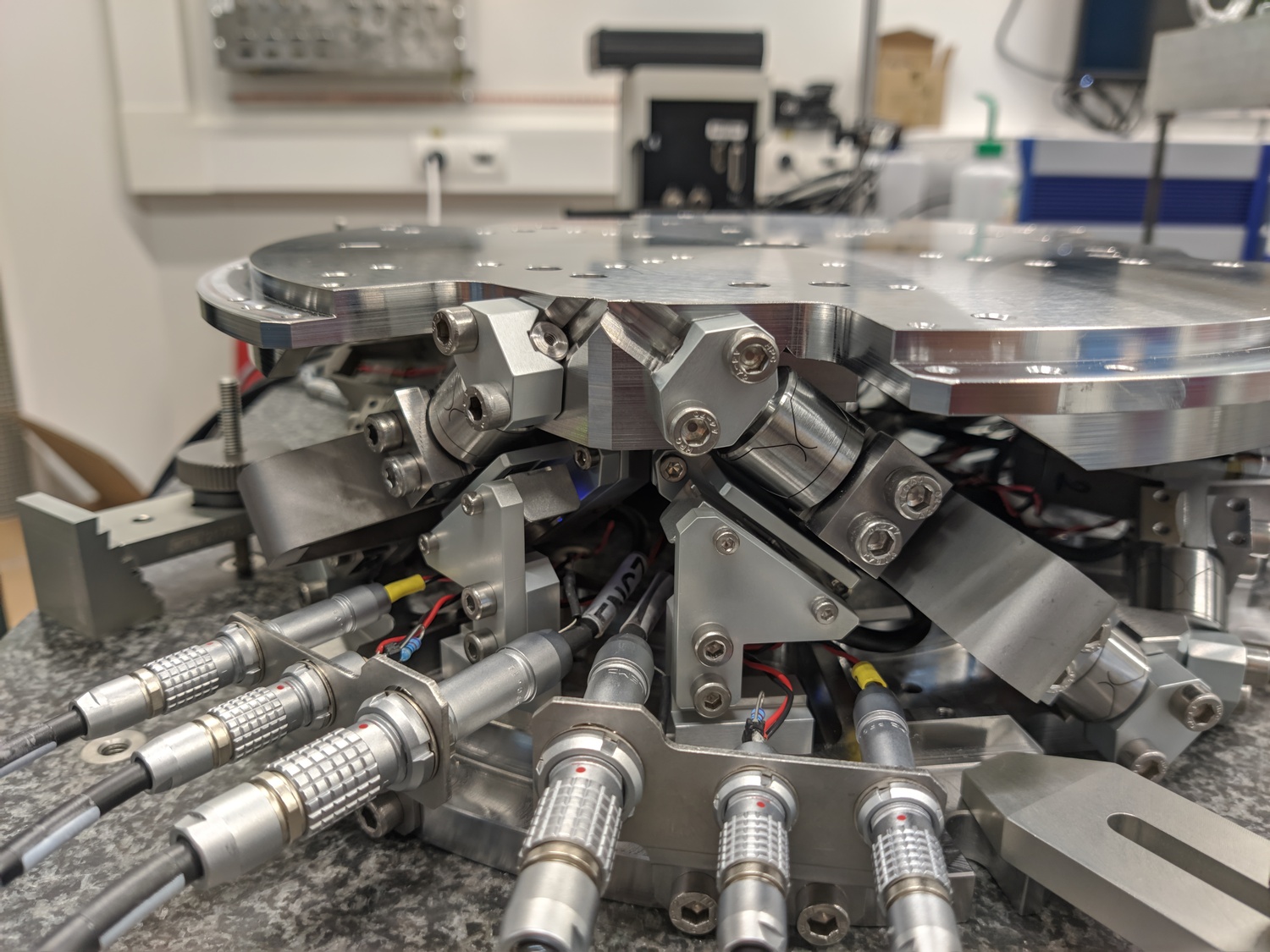
Figure 33: Nano-Hexapod with encoders fixed to the struts

It is structured as follow:

Section 2.1: The dynamics of the nano-hexapod is identified.
Section 2.2: The identified dynamics is compared with the Simscape model.
Section 2.3: The Integral Force Feedback (IFF) control strategy is applied and the dynamics of the damped nano-hexapod is identified and compare with the Simscape model.

2.1. Identification of the dynamics

In this section, the dynamics of the nano-hexapod with the encoders fixed to the plates is identified.

First, the measurement data are loaded in Section 2.1.1, then the transfer function matrix from the actuators to the encoders are estimated in Section 2.1.2. Finally, the transfer function matrix from the actuators to the force sensors is estimated in Section 2.1.3.

2.1.1. Data Loading and Spectral Analysis Setup

The actuators are excited one by one using a low pass filtered white noise. For each excitation, the 6 force sensors and 6 encoders are measured and saved.

Copy
%% Load Identification Data
meas_data_lf = {};

for i = 1:6
    meas_data_lf(i) = {load(sprintf('mat/frf_exc_strut_%i_enc_plates_noise.mat', i), 't', 'Va', 'Vs', 'de')};
end

2.1.2. Transfer function from Actuator to Encoder

Let’s compute the coherence from the excitation voltage $u$ and the displacement $d L_{m}$ as measured by the encoders.

Copy
%% Coherence
coh_dvf = zeros(length(f), 6, 6);

for i = 1:6
    coh_dvf(:, :, i) = mscohere(meas_data_lf{i}.Va, meas_data_lf{i}.de, win, [], [], 1/Ts);
end

The obtained coherence shown in Figure 34 is quite good up to 400Hz.

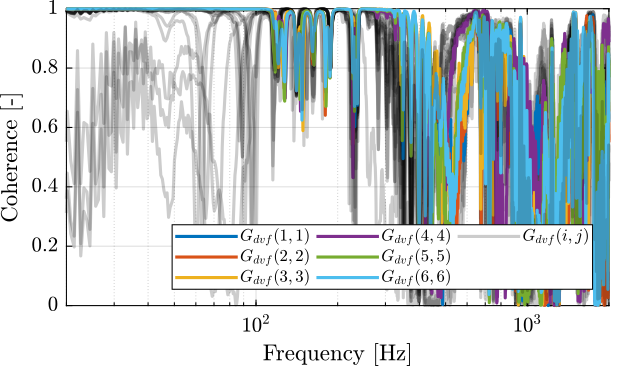
Figure 34: Obtained coherence for the DVF plant

Then the 6x6 transfer function matrix is estimated.

Copy
%% DVF Plant (transfer function from u to dLm)
G_dvf = zeros(length(f), 6, 6);

for i = 1:6
    G_dvf(:,:,i) = tfestimate(meas_data_lf{i}.Va, meas_data_lf{i}.de, win, [], [], 1/Ts);
end

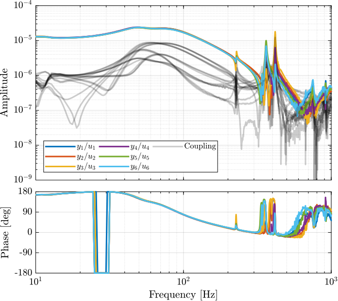
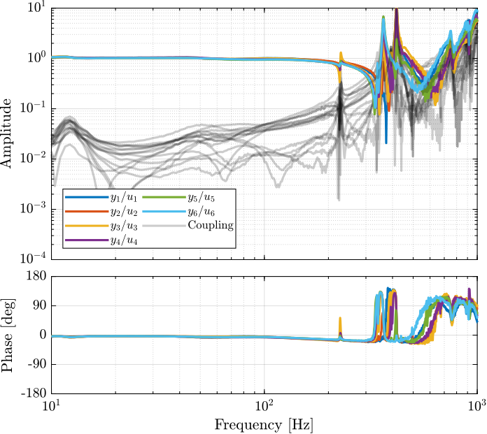
The diagonal and off-diagonal terms of this transfer function matrix are shown in Figure 35.

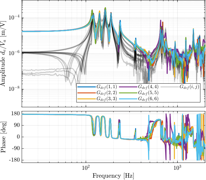
Figure 35: Measured FRF for the DVF plant

Important

From Figure 35, we can draw few conclusions on the transfer functions from $u$ to $d L_{m}$ when the encoders are fixed to the plates:

the decoupling is rather good at low frequency (below the first suspension mode). The low frequency gain is constant for the off diagonal terms, whereas when the encoders where fixed to the struts, the low frequency gain of the off-diagonal terms were going to zero (Figure 5).
the flexible modes of the struts at 226Hz and 337Hz are indeed shown in the transfer functions, but their amplitudes are rather low.
the diagonal terms have alternating poles and zeros up to at least 600Hz: the flexible modes of the struts are not affecting the alternating pole/zero pattern. This what not the case when the encoders were fixed to the struts (Figure 5).

2.1.3. Transfer function from Actuator to Force Sensor

Let’s now compute the coherence from the excitation voltage $u$ and the voltage $τ_{m}$ generated by the Force senors.

Copy
%% Coherence for the IFF plant
coh_iff = zeros(length(f), 6, 6);

for i = 1:6
    coh_iff(:,:,i) = mscohere(meas_data_lf{i}.Va, meas_data_lf{i}.Vs, win, [], [], 1/Ts);
end

The coherence is shown in Figure 36, and is very good for from 10Hz up to 2kHz.

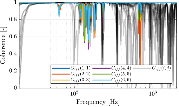
Figure 36: Obtained coherence for the IFF plant

Then the 6x6 transfer function matrix is estimated.

Copy
%% IFF Plant
G_iff = zeros(length(f), 6, 6);

for i = 1:6
    G_iff(:,:,i) = tfestimate(meas_data_lf{i}.Va, meas_data_lf{i}.Vs, win, [], [], 1/Ts);
end

The bode plot of the diagonal and off-diagonal terms are shown in Figure 37.

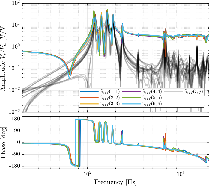
Figure 37: Measured FRF for the IFF plant

Important

It is shown in Figure 38 that:

The IFF plant has alternating poles and zeros
The first flexible mode of the struts as 235Hz is appearing, and therefore is should be possible to add some damping to this mode using IFF
The decoupling is quite good at low frequency (below the first model) as well as high frequency (above the last suspension mode, except near the flexible modes of the top plate)

2.1.4. Save Identified Plants

The identified dynamics is saved for further use.

Copy
save('mat/identified_plants_enc_plates.mat', 'f', 'Ts', 'G_iff', 'G_dvf')

2.2. Comparison with the Simscape Model

In this section, the measured dynamics done in Section 2.1 is compared with the dynamics estimated from the Simscape model.

2.2.1. Identification Setup

The nano-hexapod is initialized with the APA taken as flexible models.

Copy
%% Initialize Nano-Hexapod
n_hexapod = initializeNanoHexapodFinal('flex_bot_type', '4dof', ...
                                       'flex_top_type', '4dof', ...
                                       'motion_sensor_type', 'plates', ...
                                       'actuator_type', 'flexible');

2.2.2. Dynamics from Actuator to Force Sensors

Then the transfer function from $u$ to $τ_{m}$ is identified using the Simscape model.

Copy
%% Identify the IFF Plant (transfer function from u to taum)
clear io; io_i = 1;
io(io_i) = linio([mdl, '/du'], 1, 'openinput');   io_i = io_i + 1; % Actuator Inputs
io(io_i) = linio([mdl, '/Fm'], 1, 'openoutput'); io_i = io_i + 1; % Force Sensors

Giff = exp(-s*Ts)*linearize(mdl, io, 0.0, options);

The identified dynamics is compared with the measured FRF:

Figure 38: the individual transfer function from $u_{1}$ (the DAC voltage for the first actuator) to the force sensors of all 6 struts are compared
Figure 39: all the diagonal elements are compared
Figure 40: all the off-diagonal elements are compared

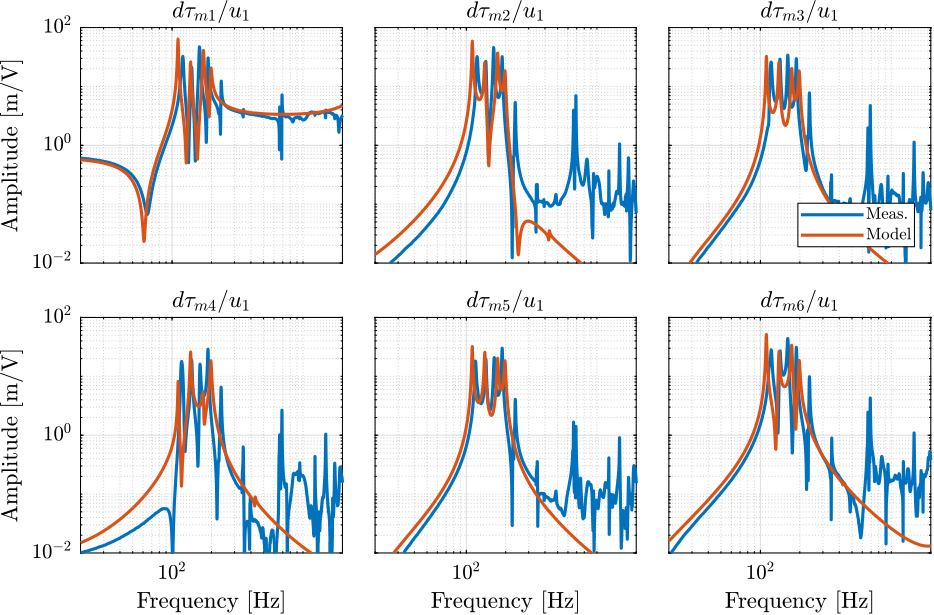
Figure 38: IFF Plant for the first actuator input and all the force senosrs

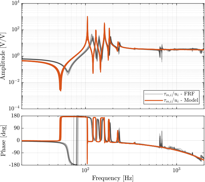
Figure 39: Diagonal elements of the IFF Plant

Figure 40: Off diagonal elements of the IFF Plant

2.2.3. Dynamics from Actuator to Encoder

Now, the dynamics from the DAC voltage $u$ to the encoders $d L_{m}$ is estimated using the Simscape model.

Copy
%% Identify the DVF Plant (transfer function from u to dLm)
clear io; io_i = 1;
io(io_i) = linio([mdl, '/du'],  1, 'openinput');  io_i = io_i + 1; % Actuator Inputs
io(io_i) = linio([mdl, '/dL'], 1, 'openoutput'); io_i = io_i + 1; % Encoders

Gdvf = exp(-s*Ts)*linearize(mdl, io, 0.0, options);

The identified dynamics is compared with the measured FRF:

Figure 41: the individual transfer function from $u_{3}$ (the DAC voltage for the actuator number 3) to the six encoders
Figure 42: all the diagonal elements are compared
Figure 43: all the off-diagonal elements are compared

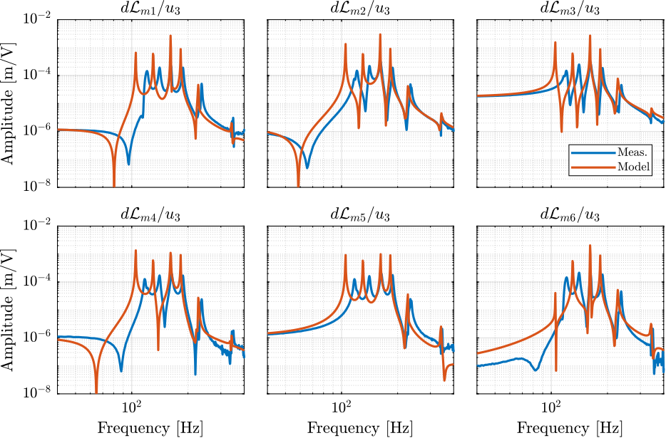
Figure 41: DVF Plant for the first actuator input and all the encoders

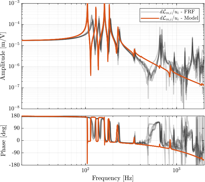
Figure 42: Diagonal elements of the DVF Plant

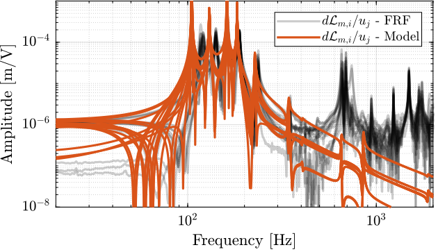
Figure 43: Off diagonal elements of the DVF Plant

2.2.4. Flexible Top Plate

Copy
%% Initialize Nano-Hexapod
n_hexapod = initializeNanoHexapodFinal('flex_bot_type', '2dof', ...
                                       'flex_top_type', '3dof', ...
                                       'motion_sensor_type', 'struts', ...
                                       'actuator_type', '2dof', ...
                                       'top_plate_type', 'rigid');

Copy
%% Identify the DVF Plant (transfer function from u to dLm)
clear io; io_i = 1;
io(io_i) = linio([mdl, '/du'],  1, 'openinput');  io_i = io_i + 1; % Actuator Inputs
io(io_i) = linio([mdl, '/dL'], 1, 'openoutput'); io_i = io_i + 1; % Encoders

Gdvf = linearize(mdl, io, 0.0, options);

Copysize(Gdvf)
isstable(Gdvf)

Copy
[sys,g] = balreal(Gdvf);  % Compute balanced realization
elim = (g<1e-4);         % Small entries of g are negligible states
rsys = modred(sys,elim); % Remove negligible states
size(rsys)

Copy
%% Identify the IFF Plant (transfer function from u to taum)
clear io; io_i = 1;
io(io_i) = linio([mdl, '/du'], 1, 'openinput');   io_i = io_i + 1; % Actuator Inputs
io(io_i) = linio([mdl, '/Fm'], 1, 'openoutput'); io_i = io_i + 1; % Force Sensors

Giff = exp(-s*Ts)*linearize(mdl, io, 0.0, options);

2.2.5. Conclusion

Important

The Simscape model is quite accurate for the transfer function matrices from $u$ to $τ_{m}$ and from $u$ to $d L_{m}$ except at frequencies of the flexible modes of the top-plate. The Simscape model can therefore be used to develop the control strategies.

2.3. Integral Force Feedback

In this section, the Integral Force Feedback (IFF) control strategy is applied to the nano-hexapod in order to add damping to the suspension modes.

The control architecture is shown in Figure 44:

$τ_{m}$ is the measured voltage of the 6 force sensors
$K_{IFF}$ is the $6 \times 6$ diagonal controller
$u$ is the plant input (voltage generated by the 6 DACs)
$u^{'}$ is the new plant inputs with added damping

Figure 44: Integral Force Feedback Strategy

Section 2.3.1

2.3.1. Effect of IFF on the plant - Simscape Model

The nano-hexapod is initialized with flexible APA and the encoders fixed to the struts.

Copy
%% Initialize the Simscape model in closed loop
n_hexapod = initializeNanoHexapodFinal('flex_bot_type', '4dof', ...
                                       'flex_top_type', '4dof', ...
                                       'motion_sensor_type', 'plates', ...
                                       'actuator_type', 'flexible');

The same controller as the one developed when the encoder were fixed to the struts is used.

Copy
%% Optimal IFF controller
load('Kiff.mat', 'Kiff')

The transfer function from $u^{'}$ to $d L_{m}$ is identified.

Copy
%% Identify the (damped) transfer function from u to dLm for different values of the IFF gain
clear io; io_i = 1;
io(io_i) = linio([mdl, '/du'],  1, 'openinput');  io_i = io_i + 1; % Actuator Inputs
io(io_i) = linio([mdl, '/dL'], 1, 'openoutput'); io_i = io_i + 1; % Plate Displacement (encoder)

First in Open-Loop:

Copy
%% Transfer function from u to dL (open-loop)
Gd_ol = exp(-s*Ts)*linearize(mdl, io, 0.0, options);

And then with the IFF controller:

Copy
%% Initialize the Simscape model in closed loop
n_hexapod = initializeNanoHexapodFinal('flex_bot_type', '4dof', ...
                                       'flex_top_type', '4dof', ...
                                       'motion_sensor_type', 'plates', ...
                                       'actuator_type', 'flexible', ...
                                       'controller_type', 'iff');

%% Transfer function from u to dL (IFF)
Gd_iff = exp(-s*Ts)*linearize(mdl, io, 0.0, options);

It is first verified that the system is stable:

Copyisstable(Gd_iff)

The diagonal and off-diagonal terms of the $6 \times 6$ transfer function matrices identified are compared in Figure 45. It is shown, as was the case when the encoders were fixed to the struts, that the IFF control strategy is very effective in damping the suspension modes of the nano-hexapod.

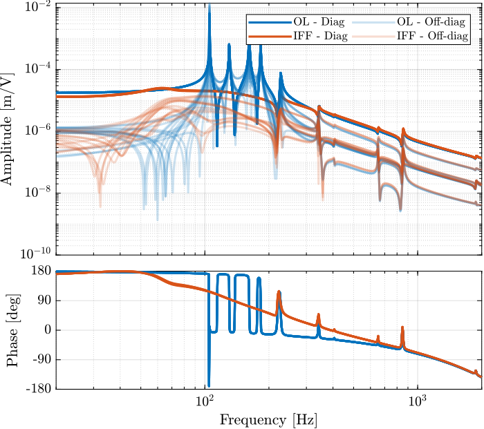
Figure 45: Effect of the IFF control strategy on the transfer function from $τ$ to $d L_{m}$

2.3.2. Effect of IFF on the plant - FRF

The IFF control strategy is experimentally implemented. The (damped) transfer function from $u^{'}$ to $d L_{m}$ is experimentally identified.

The identification data are loaded:

Copy
%% Load Identification Data
meas_iff_plates = {};

for i = 1:6
    meas_iff_plates(i) = {load(sprintf('mat/frf_exc_iff_strut_%i_enc_plates_noise.mat', i), 't', 'Va', 'Vs', 'de', 'u')};
end

And the parameters used for the transfer function estimation are defined below.

Copy
% Sampling Time [s]
Ts = (meas_iff_plates{1}.t(end) - (meas_iff_plates{1}.t(1)))/(length(meas_iff_plates{1}.t)-1);

% Hannning Windows
win = hanning(ceil(1/Ts));

% And we get the frequency vector
[~, f] = tfestimate(meas_iff_plates{1}.Va, meas_iff_plates{1}.de, win, [], [], 1/Ts);

The estimation is performed using the tfestimate command.

Copy
%% Estimation of the transfer function matrix from u to dL when IFF is applied
G_enc_iff_opt = zeros(length(f), 6, 6);

for i = 1:6
    G_enc_iff_opt(:,:,i) = tfestimate(meas_iff_plates{i}.Va, meas_iff_plates{i}.de, win, [], [], 1/Ts);
end

The obtained diagonal and off-diagonal elements of the transfer function from $u^{'}$ to $d L_{m}$ are shown in Figure 46 both without and with IFF.

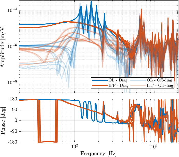
Figure 46: Effect of the IFF control strategy on the transfer function from $τ$ to $d L_{m}$

Important

As was predicted with the Simscape model, the IFF control strategy is very effective in damping the suspension modes of the nano-hexapod. Little damping is also applied on the first flexible mode of the strut at 235Hz. However, no damping is applied on other modes, such as the flexible modes of the top plate.

2.3.3. Comparison of the measured FRF and the Simscape model

Let’s now compare the obtained damped plants obtained experimentally with the one extracted from Simscape:

Figure 47: the individual transfer function from $u_{1}^{'}$ to the six encoders are comapred
Figure 48: all the diagonal elements are compared
Figure 49: all the off-diagonal elements are compared

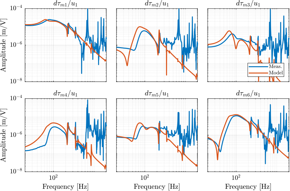
Figure 47: FRF from one actuator to all the encoders when the plant is damped using IFF

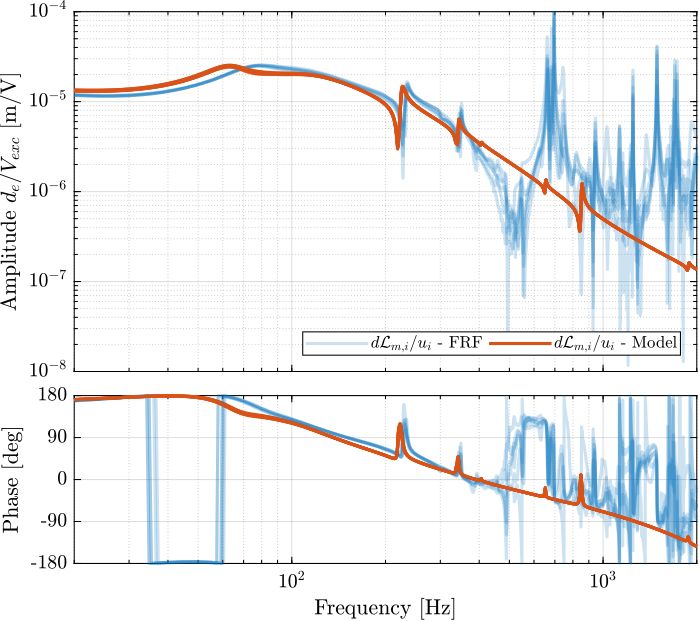
Figure 48: Comparison of the diagonal elements of the transfer functions from $u$ to $d L_{m}$ with active damping (IFF) applied with an optimal gain $g = 400$

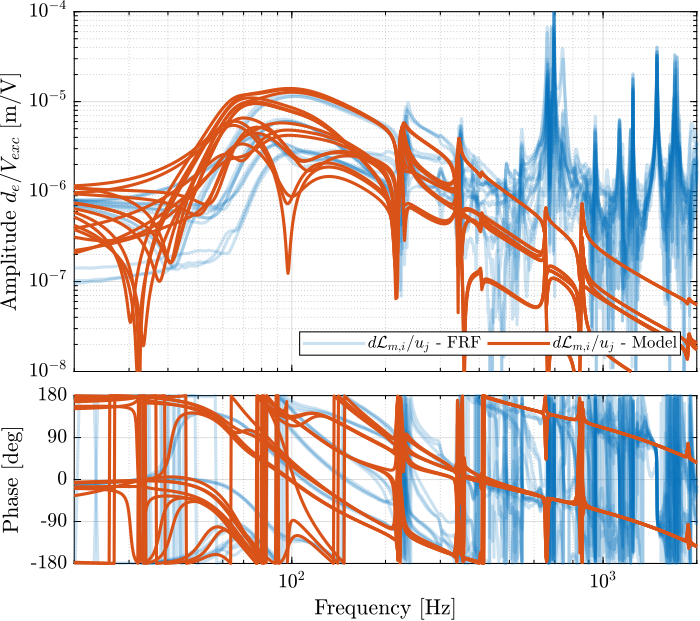
Figure 49: Comparison of the off-diagonal elements of the transfer functions from $u$ to $d L_{m}$ with active damping (IFF) applied with an optimal gain $g = 400$

Important

From Figures 48 and 49, it is clear that the Simscape model very well represents the dynamics of the nano-hexapod. This is true to around 400Hz, then the dynamics depends on the flexible modes of the top plate which are not modelled.

2.3.4. Save Damped Plant

The experimentally identified plant is saved for further use.

Copy
save('matlab/mat/damped_plant_enc_plates.mat', 'f', 'Ts', 'G_enc_iff_opt')

Copy
save('mat/damped_plant_enc_plates.mat', 'f', 'Ts', 'G_enc_iff_opt')

2.4. Effect of Payload mass - Robust IFF

In this section, the encoders are fixed to the plates, and we identify the dynamics for several payloads. The added payload are half cylinders, and three layers can be added for a total of around 40kg (Figure 50).

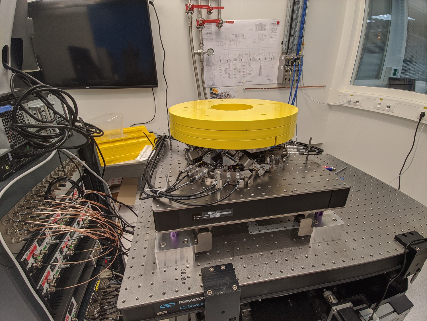
Figure 50: Picture of the nano-hexapod with added mass

First the dynamics from $u$ to $d L_{m}$ and $τ_{m}$ is identified. Then, the Integral Force Feedback controller is developed and applied as shown in Figure 51. Finally, the dynamics from $u^{'}$ to $d L_{m}$ is identified and the added damping can be estimated.

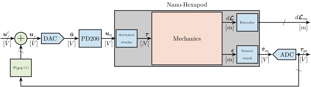
Figure 51: Block Diagram of the experimental setup and model

2.4.1. Measured Frequency Response Functions

2.4.1.1. Compute FRF in open-loop

The identification is performed without added mass, and with one, two and three layers of added cylinders.

Copy
i_masses = 0:3;

The following data are loaded:

Va: the excitation voltage (corresponding to $u_{i}$ )
Vs: the generated voltage by the 6 force sensors (corresponding to $τ_{m}$ )
de: the measured motion by the 6 encoders (corresponding to $d L_{m}$ )

Copy
%% Load Identification Data
meas_added_mass = {};

for i_mass = i_masses
    for i_strut = 1:6
        meas_added_mass(i_strut, i_mass+1) = {load(sprintf('frf_data_exc_strut_%i_realigned_vib_table_%im.mat', i_strut, i_mass), 't', 'Va', 'Vs', 'de')};
    end
end

The window win and the frequency vector f are defined.

Copy
% Sampling Time [s]
Ts = (meas_added_mass{1,1}.t(end) - (meas_added_mass{1,1}.t(1)))/(length(meas_added_mass{1,1}.t)-1);

% Hannning Windows
win = hanning(ceil(1/Ts));

% And we get the frequency vector
[~, f] = tfestimate(meas_added_mass{1,1}.Va, meas_added_mass{1,1}.de, win, [], [], 1/Ts);

Finally the $6 \times 6$ transfer function matrices from $u$ to $d L_{m}$ and from $u$ to $τ_{m}$ are identified:

Copy
%% DVF Plant (transfer function from u to dLm)
G_dL = {};

for i_mass = i_masses
    G_dL(i_mass+1) = {zeros(length(f), 6, 6)};
    for i_strut = 1:6
        G_dL{i_mass+1}(:,:,i_strut) = tfestimate(meas_added_mass{i_strut, i_mass+1}.Va, meas_added_mass{i_strut, i_mass+1}.de, win, [], [], 1/Ts);
    end
end

%% IFF Plant (transfer function from u to taum)
G_tau = {};

for i_mass = i_masses
    G_tau(i_mass+1) = {zeros(length(f), 6, 6)};
    for i_strut = 1:6
        G_tau{i_mass+1}(:,:,i_strut) = tfestimate(meas_added_mass{i_strut, i_mass+1}.Va, meas_added_mass{i_strut, i_mass+1}.Vs, win, [], [], 1/Ts);
    end
end

The identified dynamics are then saved for further use.

Copy
save('mat/frf_vib_table_m.mat', 'f', 'Ts', 'G_tau', 'G_dL')

2.4.2. Transfer function from $u$ to $d L_{m}$

The transfer functions from $u_{i}$ to $d L_{m, i}$ are shown in Figure 52.

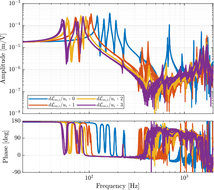
Figure 52: Measured Frequency Response Functions from $u_{i}$ to $d L_{m, i}$ for all 4 payload conditions

Important

From Figure 52, we can observe few things:

The obtained dynamics is changing a lot between the case without mass and when there is at least one added mass.
Between 1, 2 and 3 added masses, the dynamics is not much different, and it would be easier to design a controller only for these cases.
The flexible modes of the top plate is first decreased a lot when the first mass is added (from 700Hz to 400Hz). This is due to the fact that the added mass is composed of two half cylinders which are not fixed together. Therefore is adds a lot of mass to the top plate without adding a lot of rigidity in one direction. When more than 1 mass layer is added, the half cylinders are added with some angles such that rigidity are added in all directions (see Figure 50). In that case, the frequency of these flexible modes are increased. In practice, the payload should be one solid body, and we should not see a massive decrease of the frequency of this flexible mode.
Flexible modes of the top plate are becoming less problematic as masses are added.
First flexible mode of the strut at 230Hz is not much decreased when mass is added. However, its apparent amplitude is much decreased.

2.4.3. Transfer function from $u$ to $τ_{m}$

The transfer functions from $u_{i}$ to $τ_{m, i}$ are shown in Figure 53.

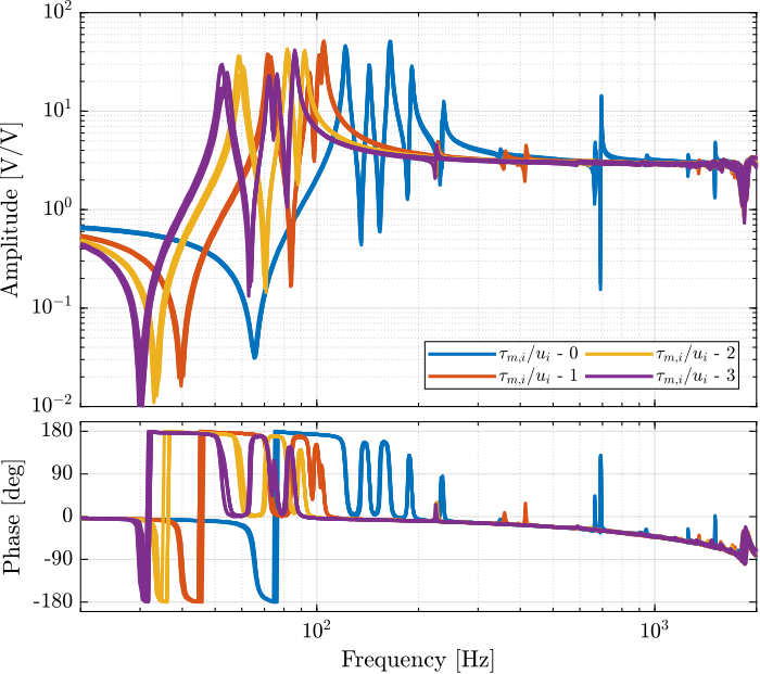
Figure 53: Measured Frequency Response Functions from $u_{i}$ to $τ_{m, i}$ for all 4 payload conditions

Important

From Figure 53, we can see that for all added payloads, the transfer function from $u_{i}$ to $τ_{m, i}$ always has alternating poles and zeros.

2.5. Comparison with the Simscape model

2.5.1. System Identification

Let’s initialize the simscape model with the nano-hexapod fixed on top of the vibration table.

Copy
support.type = 1; % On top of vibration table

The model of the nano-hexapod is defined as shown bellow:

Copy
%% Initialize Nano-Hexapod
n_hexapod = initializeNanoHexapodFinal('flex_bot_type', '2dof', ...
                                       'flex_top_type', '3dof', ...
                                       'motion_sensor_type', 'plates', ...
                                       'actuator_type', '2dof');

And finally, we add the same payloads as during the experiments:

Copy
payload.type = 1; % Payload / 1 "mass layer"

First perform the identification for the transfer functions from $u$ to $d L_{m}$ :

Copy
%% Identify the DVF Plant (transfer function from u to dLm)
clear io; io_i = 1;
io(io_i) = linio([mdl, '/du'], 1, 'openinput');  io_i = io_i + 1; % Actuator Inputs
io(io_i) = linio([mdl, '/dL'], 1, 'openoutput'); io_i = io_i + 1; % Encoders

%% Identification for all the added payloads
G_dL = {};

for i = i_masses
    fprintf('i = %i\n', i)
    payload.type = i;
    G_dL(i+1) = {exp(-s*frf_ol.Ts)*linearize(mdl, io, 0.0, options)};
end

Copy
%% Identify the IFF Plant (transfer function from u to taum)
clear io; io_i = 1;
io(io_i) = linio([mdl, '/du'], 1, 'openinput');  io_i = io_i + 1; % Actuator Inputs
io(io_i) = linio([mdl, '/Fm'], 1, 'openoutput'); io_i = io_i + 1; % Force Sensors

%% Identification for all the added payloads
G_tau = {};

for i = 0:3
    fprintf('i = %i\n', i)
    payload.type = i;
    G_tau(i+1) = {exp(-s*frf_ol.Ts)*linearize(mdl, io, 0.0, options)};
end

The identified dynamics are then saved for further use.

Copy
save('mat/sim_vib_table_m.mat', 'G_tau', 'G_dL')

2.5.2. Transfer function from $u$ to $d L_{m}$

The measured FRF and the identified dynamics from $u_{i}$ to $d L_{m, i}$ are compared in Figure 54. A zoom near the “suspension” modes is shown in Figure 55.

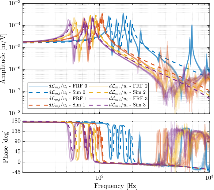
Figure 54: Comparison of the transfer functions from $u_{i}$ to $d L_{m, i}$ - measured FRF and identification from the Simscape model

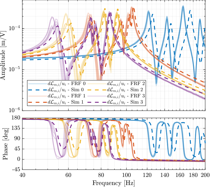
Figure 55: Comparison of the transfer functions from $u_{i}$ to $d L_{m, i}$ - measured FRF and identification from the Simscape model (Zoom)

Important

The Simscape model is very accurately representing the measured dynamics up. Only the flexible modes of the struts and of the top plate are not represented here as these elements are modelled as rigid bodies.

2.5.3. Transfer function from $u$ to $τ_{m}$

The measured FRF and the identified dynamics from $u_{i}$ to $τ_{m, i}$ are compared in Figure 56. A zoom near the “suspension” modes is shown in Figure 57.

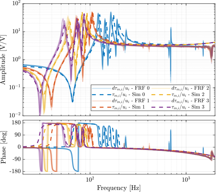
Figure 56: Comparison of the transfer functions from $u_{i}$ to $τ_{m, i}$ - measured FRF and identification from the Simscape model

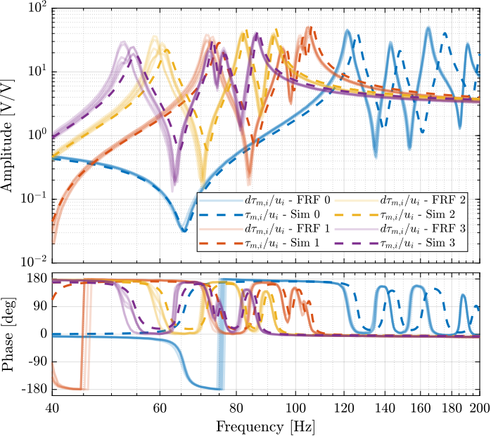
Figure 57: Comparison of the transfer functions from $u_{i}$ to $τ_{m, i}$ - measured FRF and identification from the Simscape model (Zoom)

2.6. Integral Force Feedback Controller

2.6.1. Robust IFF Controller

Based on the measured FRF from $u_{i}$ to $τ_{m, i}$ , the following IFF controller is developed:

Copy
%% IFF Controller
Kiff_g1 = (1/(s + 2*pi*20))*... % LPF: provides integral action above 20[Hz]
          (s/(s + 2*pi*20))*... % HPF: limit low frequency gain
          (1/(1 + s/2/pi/400)); % LPF: more robust to high frequency resonances

Then, the Root Locus plot of Figure 58 is used to estimate the optimal gain. This Root Locus plot is computed from the Simscape model.

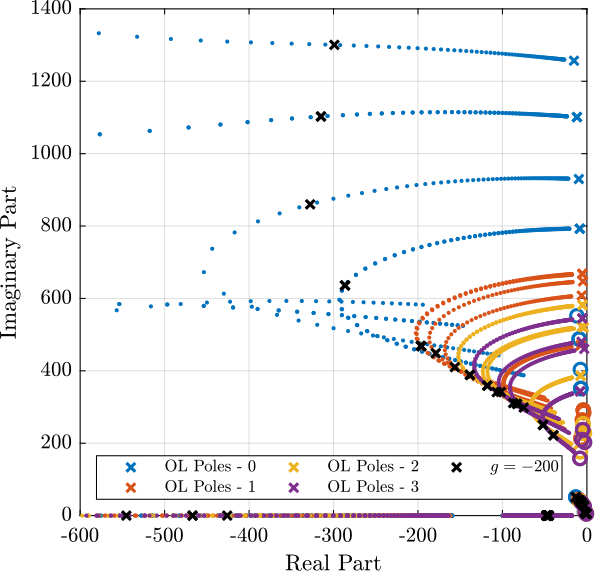
Figure 58: Root Locus for the IFF control strategy (for all payload conditions).

The found optimal IFF controller is:

Copy
%% Optimal controller
g_opt = -2e2;
Kiff = g_opt*Kiff_g1*eye(6);

It is saved for further use.

Copy
save('mat/Kiff_opt.mat', 'Kiff')

The corresponding experimental loop gains are shown in Figure 59.

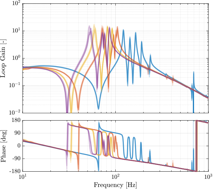
Figure 59: Loop gain for the Integral Force Feedback controller

Important

Based on the above analysis:

The same IFF controller can be used to damp the suspension modes for all payload conditions
The IFF controller should be robust

2.6.2. Estimated Damped Plant from the Simscape model

Let’s initialize the simscape model with the nano-hexapod fixed on top of the vibration table.

Copy
support.type = 1; % On top of vibration table

The model of the nano-hexapod is defined as shown bellow:

Copy
%% Initialize the Simscape model in closed loop
n_hexapod = initializeNanoHexapodFinal('flex_bot_type', '2dof', ...
                                       'flex_top_type', '3dof', ...
                                       'motion_sensor_type', 'plates', ...
                                       'actuator_type', '2dof', ...
                                       'controller_type', 'iff');

And finally, we add the same payloads as during the experiments:

Copy
payload.type = 1; % Payload / 1 "mass layer"

Copy
%% Identify the (damped) transfer function from u to dLm
clear io; io_i = 1;
io(io_i) = linio([mdl, '/du'], 1, 'openinput');  io_i = io_i + 1; % Actuator Inputs
io(io_i) = linio([mdl, '/dL'], 1, 'openoutput'); io_i = io_i + 1; % Plate Displacement (encoder)

%% Identify for all add masses
G_dL = {};

for i = i_masses
    payload.type = i;
    G_dL(i+1) = {exp(-s*frf_ol.Ts)*linearize(mdl, io, 0.0, options)};
end

The identified dynamics are then saved for further use.

Copy
save('mat/sim_iff_vib_table_m.mat', 'G_dL');

Copy
sim_iff = load('sim_iff_vib_table_m.mat', 'G_dL');

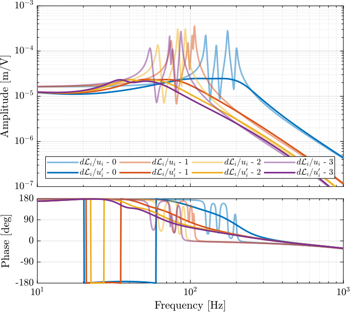
Figure 60: Transfer function from $u_{i}$ to $d L_{m, i}$ (without active damping) and from $u_{i}^{'}$ to $d L_{m, i}$ (with IFF)

2.6.3. Compute the identified FRF with IFF

The identification is performed without added mass, and with one, two and three layers of added cylinders.

Copy
i_masses = 0:3;

The following data are loaded:

Va: the excitation voltage for the damped plant (corresponding to $u_{i}^{'}$ )
de: the measured motion by the 6 encoders (corresponding to $d L_{m}$ )

Copy
%% Load Identification Data
meas_added_mass = {};

for i_mass = i_masses
    for i_strut = 1:6
        meas_iff_mass(i_strut, i_mass+1) = {load(sprintf('frf_data_exc_strut_%i_iff_vib_table_%im.mat', i_strut, i_mass), 't', 'Va', 'de')};
    end
end

The window win and the frequency vector f are defined.

Copy
% Sampling Time [s]
Ts = (meas_iff_mass{1,1}.t(end) - (meas_iff_mass{1,1}.t(1)))/(length(meas_iff_mass{1,1}.t)-1);

% Hannning Windows
win = hanning(ceil(1/Ts));

% And we get the frequency vector
[~, f] = tfestimate(meas_iff_mass{1,1}.Va, meas_iff_mass{1,1}.de, win, [], [], 1/Ts);

Finally the $6 \times 6$ transfer function matrix from $u^{'}$ to $d L_{m}$ is estimated:

Copy
%% DVF Plant (transfer function from u to dLm)
G_dL = {};

for i_mass = i_masses
    G_dL(i_mass+1) = {zeros(length(f), 6, 6)};
    for i_strut = 1:6
        G_dL{i_mass+1}(:,:,i_strut) = tfestimate(meas_iff_mass{i_strut, i_mass+1}.Va, meas_iff_mass{i_strut, i_mass+1}.de, win, [], [], 1/Ts);
    end
end

The identified dynamics are then saved for further use.

Copy
save('mat/frf_iff_vib_table_m.mat', 'f', 'Ts', 'G_dL');

2.6.4. Comparison of the measured FRF and the Simscape model

The following figures are computed:

Figure 61: the measured damped FRF are displayed
Figure 62: the open-loop and damped FRF are compared (diagonal elements)
Figure 63: the obtained damped FRF is compared with the identified damped from using the Simscape model

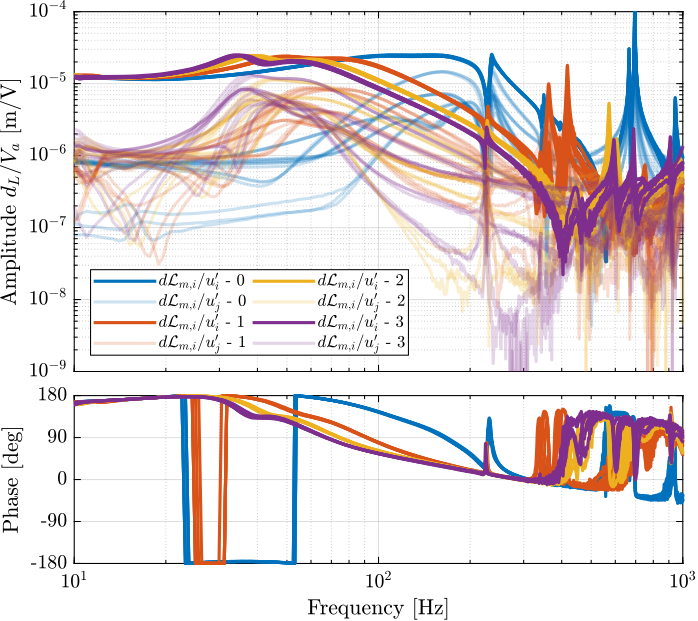
Figure 61: Diagonal and off-diagonal of the measured FRF matrix for the damped plant

Figure 62: Damped and Undamped measured FRF (diagonal elements)

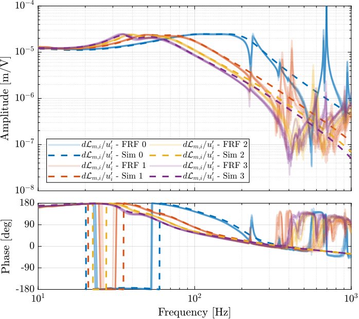
Figure 63: Comparison of the measured FRF and the identified dynamics from the Simscape model

Important

The IFF control strategy effectively damps all the suspensions modes of the nano-hexapod whatever the payload is. The obtained plant is easier to control (provided the flexible modes of the top platform are well damped).

2.6.5. Change of coupling with IFF

The added damping using IFF reduces the coupling in the system near the suspensions modes that are damped. It can be estimated by taking the ratio of the diagonal-term and the off-diagonal term.

This is shown in Figure 64.

Figure 64: Comparison of the coupling with and without IFF

2.7. Un-Balanced mass

2.7.1. Introduction

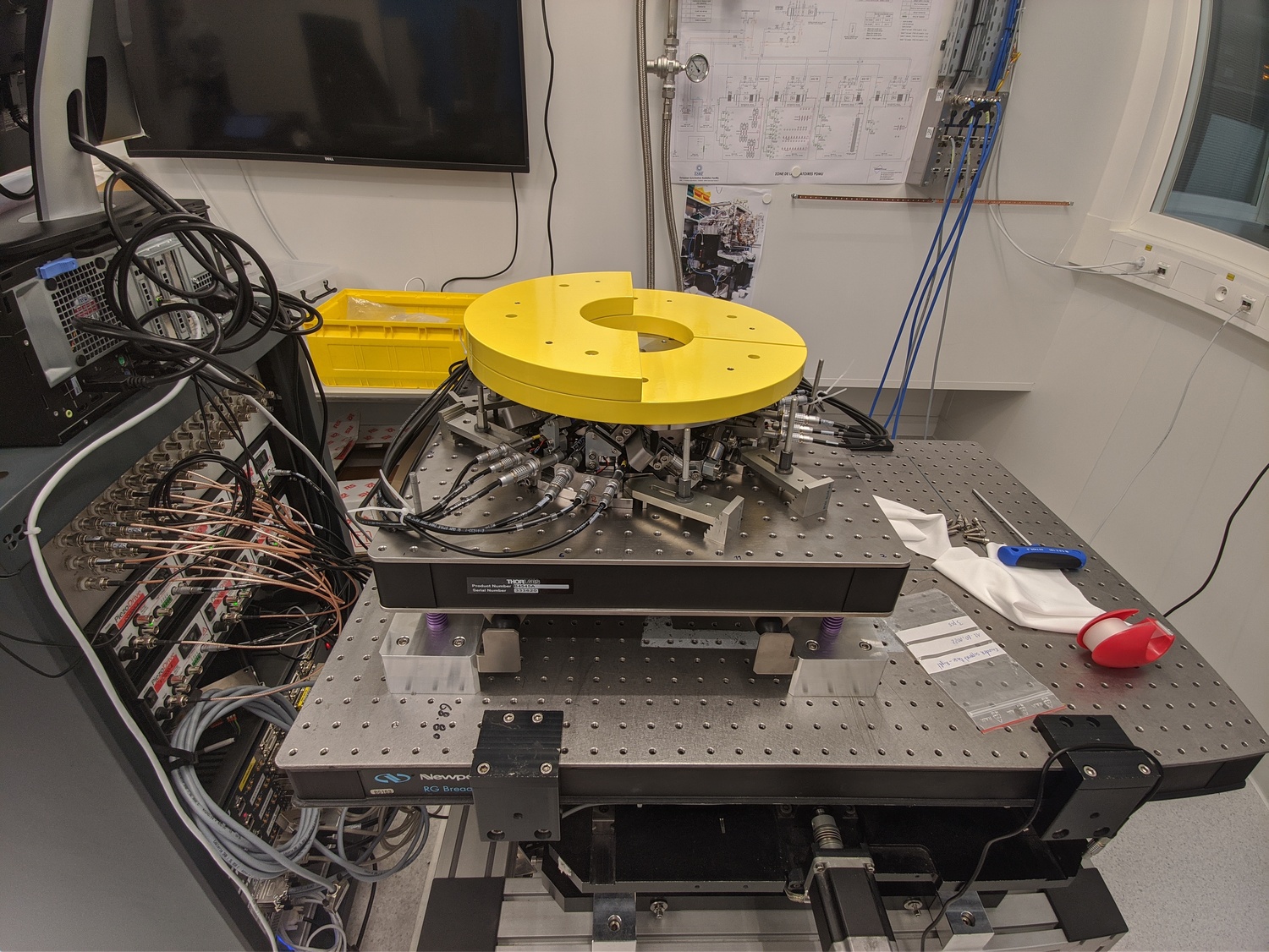
Figure 65: Nano-Hexapod with unbalanced payload

2.7.2. Compute the identified FRF with IFF

The following data are loaded:

Va: the excitation voltage for the damped plant (corresponding to $u_{i}^{'}$ )
de: the measured motion by the 6 encoders (corresponding to $d L_{m}$ )

Copy
%% Load Identification Data
meas_added_mass = {zeros(6,1)};

for i_strut = 1:6
    meas_iff_mass(i_strut) = {load(sprintf('frf_data_exc_strut_%i_iff_vib_table_1m_unbalanced.mat', i_strut), 't', 'Va', 'de')};
end

The window win and the frequency vector f are defined.

Copy
% Sampling Time [s]
Ts = (meas_iff_mass{1}.t(end) - (meas_iff_mass{1}.t(1)))/(length(meas_iff_mass{1}.t)-1);

% Hannning Windows
win = hanning(ceil(1/Ts));

% And we get the frequency vector
[~, f] = tfestimate(meas_iff_mass{1}.Va, meas_iff_mass{1}.de, win, [], [], 1/Ts);

Finally the $6 \times 6$ transfer function matrix from $u^{'}$ to $d L_{m}$ is estimated:

Copy
%% DVF Plant (transfer function from u to dLm)
G_dL = zeros(length(f), 6, 6);
for i_strut = 1:6
    G_dL(:,:,i_strut) = tfestimate(meas_iff_mass{i_strut}.Va, meas_iff_mass{i_strut}.de, win, [], [], 1/Ts);
end

The identified dynamics are then saved for further use.

Copy
save('mat/frf_iff_unbalanced_vib_table_m.mat', 'f', 'Ts', 'G_dL');

2.7.3. Effect of an unbalanced payload

The transfer functions from $u_{i}$ to $d L_{i}$ are shown in Figure 66. Due to the unbalanced payload, the system is not symmetrical anymore, and therefore each of the diagonal elements are not equal. This is due to the fact that each strut is not affected by the same inertia.

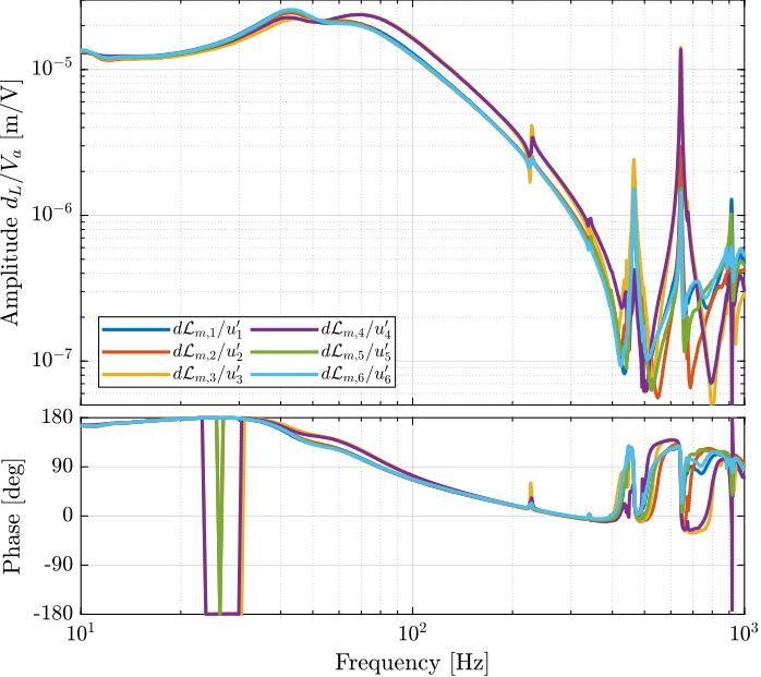
Figure 66: Transfer function from $u_{i}$ to $d L_{i}$ for the nano-hexapod with an unbalanced payload

2.8. Conclusion

Important

In this section, the dynamics of the nano-hexapod with the encoders fixed to the plates is studied.

It has been found that:

The measured dynamics is in agreement with the dynamics of the simscape model, up to the flexible modes of the top plate. See figures 39 and 40 for the transfer function to the force sensors and Figures 42 and 43for the transfer functions to the encoders
The Integral Force Feedback strategy is very effective in damping the suspension modes of the nano-hexapod (Figure 46).
The transfer function from $u^{'}$ to $d L_{m}$ show nice dynamical properties and is a much better candidate for the high-authority-control than when the encoders were fixed to the struts. At least up to the flexible modes of the top plate, the diagonal elements of the transfer function matrix have alternating poles and zeros, and the phase is moving smoothly. Only the flexible modes of the top plates seems to be problematic for control.

3. Decentralized High Authority Control with Integral Force Feedback

In this section is studied the HAC-IFF architecture for the Nano-Hexapod. More precisely:

The LAC control is a decentralized integral force feedback as studied in Section 2.3
The HAC control is a decentralized controller working in the frame of the struts

The corresponding control architecture is shown in Figure 67 with:

$r_{X_{n}}$ : the $6 \times 1$ reference signal in the cartesian frame
$r_{d L}$ : the $6 \times 1$ reference signal transformed in the frame of the struts thanks to the inverse kinematic
$ϵ_{d L}$ : the $6 \times 1$ length error of the 6 struts
$u^{'}$ : input of the damped plant
$u$ : generated DAC voltages
$τ_{m}$ : measured force sensors
$d L_{m}$ : measured displacement of the struts by the encoders

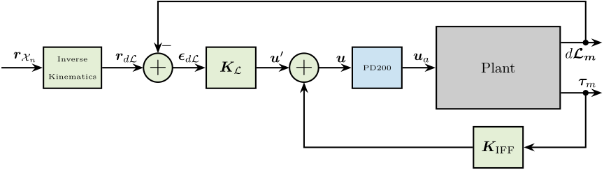
Figure 67: HAC-LAC: IFF + Control in the frame of the legs

This part is structured as follow:

Section 3.1: some reference tracking tests are performed
Section 3.2: the decentralized high authority controller is tuned using the Simscape model and is implemented and tested experimentally
Section 3.3: an interaction analysis is performed, from which the best decoupling strategy can be determined
Section 3.4: Robust High Authority Controller are designed

3.1. Reference Tracking - Trajectories

In this section, several trajectories representing the wanted pose (position and orientation) of the top platform with respect to the bottom platform are defined.

These trajectories will be used to test the HAC-LAC architecture.

In order to transform the wanted pose to the wanted displacement of the 6 struts, the inverse kinematic is required. As a first approximation, the Jacobian matrix $J$ can be used instead of using the full inverse kinematic equations.

Therefore, the control architecture with the input trajectory $r_{X_{n}}$ is shown in Figure 68.

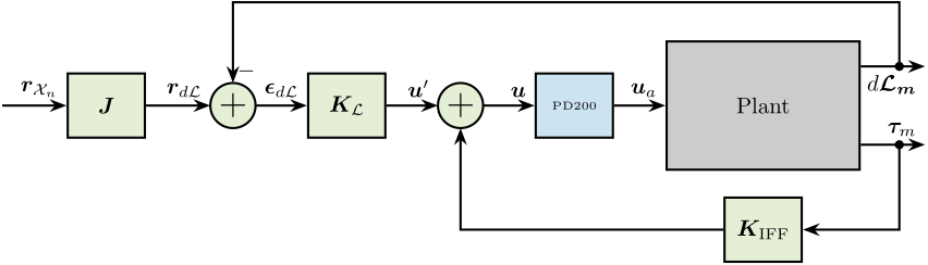
Figure 68: HAC-LAC: IFF + Control in the frame of the legs

In the following sections, several reference trajectories are defined:

Section 3.1.1: simple scans in the Y-Z plane
Section 3.1.2: scans in tilt are performed
Section 3.1.3: scans with X-Y-Z translations in order to draw the word “NASS”

3.1.1. Y-Z Scans

A function generateYZScanTrajectory has been developed (accessible here) in order to easily generate scans in the Y-Z plane.

For instance, the following generated trajectory is represented in Figure 69.

Copy
%% Generate the Y-Z trajectory scan
Rx_yz = generateYZScanTrajectory(...
    'y_tot', 4e-6, ... % Length of Y scans [m]
    'z_tot', 4e-6, ... % Total Z distance [m]
    'n', 5, ...     % Number of Y scans
    'Ts', 1e-3, ... % Sampling Time [s]
    'ti', 1, ...    % Time to go to initial position [s]
    'tw', 0, ...    % Waiting time between each points [s]
    'ty', 0.6, ...  % Time for a scan in Y [s]
    'tz', 0.2);     % Time for a scan in Z [s]

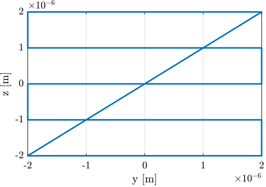
Figure 69: Generated scan in the Y-Z plane

The Y and Z positions as a function of time are shown in Figure 70.

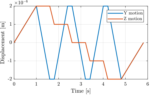
Figure 70: Y and Z trajectories as a function of time

Using the Jacobian matrix, it is possible to compute the wanted struts lengths as a function of time:

\begin{matrix} (1) & r_{d L} = J r_{X_{n}} \end{matrix}

Copy
%% Compute the reference in the frame of the legs
dL_ref = [J*Rx_yz(:, 2:7)']';

The reference signal for the strut length is shown in Figure 71.

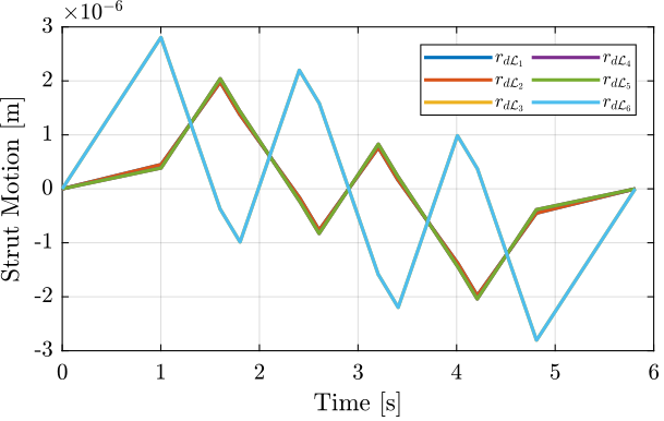
Figure 71: Trajectories for the 6 individual struts

3.1.2. Tilt Scans

A function generalSpiralAngleTrajectory has been developed in order to easily generate $R_{x}, R_{y}$ tilt scans.

For instance, the following generated trajectory is represented in Figure 72.

Copy
%% Generate the "tilt-spiral" trajectory scan
R_tilt = generateSpiralAngleTrajectory(...
    'R_tot',  20e-6, ... % Total Tilt [ad]
    'n_turn', 5, ...     % Number of scans
    'Ts',     1e-3, ...  % Sampling Time [s]
    't_turn', 1, ...     % Turn time [s]
    't_end',  1);        % End time to go back to zero [s]

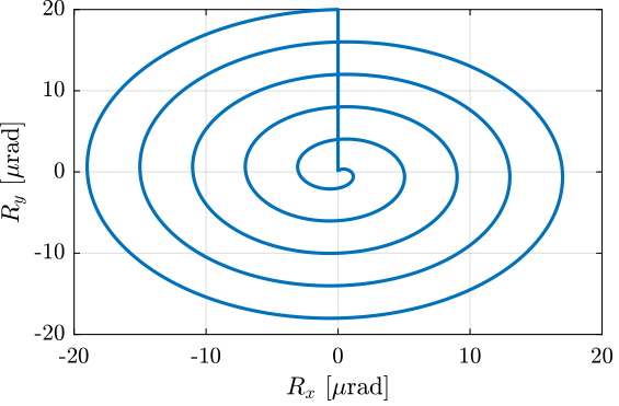
Figure 72: Generated “spiral” scan

The reference signal for the strut length is shown in Figure 73.

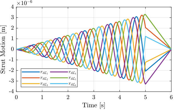
Figure 73: Trajectories for the 6 individual struts - Tilt scan

3.1.3. “NASS” reference path

In this section, a reference path that “draws” the work “NASS” is developed.

First, a series of points representing each letter are defined. Between each letter, a negative Z motion is performed.

Copy
%% List of points that draws "NASS"
ref_path = [ ...
    0, 0,0; % Initial Position
    0,0,1; 0,4,1; 3,0,1; 3,4,1; % N
    3,4,0; 4,0,0; % Transition
    4,0,1; 4,3,1; 5,4,1; 6,4,1; 7,3,1; 7,2,1; 4,2,1; 4,3,1; 5,4,1; 6,4,1; 7,3,1; 7,0,1; % A
    7,0,0; 8,0,0; % Transition
    8,0,1; 11,0,1; 11,2,1; 8,2,1; 8,4,1; 11,4,1; % S
    11,4,0; 12,0,0; % Transition
    12,0,1; 15,0,1; 15,2,1; 12,2,1; 12,4,1; 15,4,1; % S
    15,4,0;
           ];

%% Center the trajectory arround zero
ref_path = ref_path - (max(ref_path) - min(ref_path))/2;

%% Define the X-Y-Z cuboid dimensions containing the trajectory
X_max = 10e-6;
Y_max =  4e-6;
Z_max =  2e-6;

ref_path = ([X_max, Y_max, Z_max]./max(ref_path)).*ref_path; % [m]

Then, using the generateXYZTrajectory function, the $6 \times 1$ trajectory signal is computed.

Copy
%% Generating the trajectory
Rx_nass = generateXYZTrajectory('points', ref_path);

The trajectory in the X-Y plane is shown in Figure 74 (the transitions between the letters are removed).

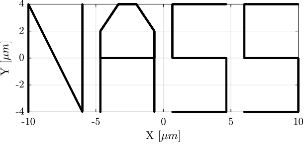
Figure 74: Reference path corresponding to the “NASS” acronym

It can also be better viewed in a 3D representation as in Figure 75.

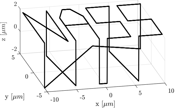
Figure 75: Reference path that draws “NASS” - 3D view

3.2. First Basic High Authority Controller

In this section, a simple decentralized high authority controller $K_{L}$ is developed to work without any payload.

The diagonal controller is tuned using classical Loop Shaping in Section 3.2.1. The stability is verified in Section 3.2.2 using the Simscape model.

3.2.1. HAC Controller

Let’s first try to design a first decentralized controller with:

a bandwidth of 100Hz
sufficient phase margin
simple and understandable components

After some very basic and manual loop shaping, A diagonal controller is developed. Each diagonal terms are identical and are composed of:

A lead around 100Hz
A first order low pass filter starting at 200Hz to add some robustness to high frequency modes
A notch at 700Hz to cancel the flexible modes of the top plate
A pure integrator

Copy
%% Lead to increase phase margin
a  = 2;  % Amount of phase lead / width of the phase lead / high frequency gain
wc = 2*pi*100; % Frequency with the maximum phase lead [rad/s]

H_lead = (1 + s/(wc/sqrt(a)))/(1 + s/(wc*sqrt(a)));

%% Low Pass filter to increase robustness
H_lpf = 1/(1 + s/2/pi/200);

%% Notch at the top-plate resonance
gm = 0.02;
xi = 0.3;
wn = 2*pi*700;

H_notch = (s^2 + 2*gm*xi*wn*s + wn^2)/(s^2 + 2*xi*wn*s + wn^2);

%% Decentralized HAC
Khac_iff_struts = -(1/(2.87e-5)) * ... % Gain
                  H_lead * ...       % Lead
                  H_notch * ...      % Notch
                  (2*pi*100/s) * ... % Integrator
                  eye(6);            % 6x6 Diagonal

This controller is saved for further use.

Copy
save('mat/Khac_iff_struts.mat', 'Khac_iff_struts')

The experimental loop gain is computed and shown in Figure 76.

Copy
L_hac_iff_struts = pagemtimes(permute(frf_iff.G_dL{1}, [2 3 1]), squeeze(freqresp(Khac_iff_struts, frf_iff.f, 'Hz')));

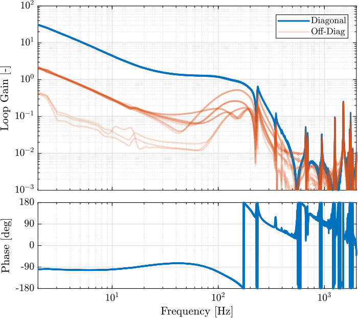
Figure 76: Diagonal and off-diagonal elements of the Loop gain for “HAC-IFF-Struts”

3.2.2. Verification of the Stability using the Simscape model

The HAC-IFF control strategy is implemented using Simscape.

Copy
%% Initialize the Simscape model in closed loop
n_hexapod = initializeNanoHexapodFinal('flex_bot_type', '4dof', ...
                                       'flex_top_type', '4dof', ...
                                       'motion_sensor_type', 'plates', ...
                                       'actuator_type', 'flexible', ...
                                       'controller_type', 'hac-iff-struts');

Copy
%% Identify the (damped) transfer function from u to dLm
clear io; io_i = 1;
io(io_i) = linio([mdl, '/du'], 1, 'openinput');  io_i = io_i + 1; % Actuator Inputs
io(io_i) = linio([mdl, '/dL'], 1, 'openoutput'); io_i = io_i + 1; % Plate Displacement (encoder)

We identify the closed-loop system.

Copy
%% Identification
Gd_iff_hac_opt = linearize(mdl, io, 0.0, options);

And verify that it is indeed stable.

Copy
%% Verify the stability
isstable(Gd_iff_hac_opt)

3.2.3. Experimental Validation

Both the Integral Force Feedback controller (developed in Section 2.3) and the high authority controller working in the frame of the struts (developed in Section 3.2) are implemented experimentally.

Two reference tracking experiments are performed to evaluate the stability and performances of the implemented control.

Copy
%% Load the experimental data
load('hac_iff_struts_yz_scans.mat', 't', 'de')

The position of the top-platform is estimated using the Jacobian matrix:

Copy
%% Pose of the top platform from the encoder values
load('jacobian.mat', 'J');
Xe = [inv(J)*de']';

Copy
%% Generate the Y-Z trajectory scan
Rx_yz = generateYZScanTrajectory(...
    'y_tot', 4e-6, ... % Length of Y scans [m]
    'z_tot', 8e-6, ... % Total Z distance [m]
    'n', 5, ...     % Number of Y scans
    'Ts', 1e-3, ... % Sampling Time [s]
    'ti', 1, ...    % Time to go to initial position [s]
    'tw', 0, ...    % Waiting time between each points [s]
    'ty', 0.6, ...  % Time for a scan in Y [s]
    'tz', 0.2);     % Time for a scan in Z [s]

The reference path as well as the measured position are partially shown in the Y-Z plane in Figure 77.

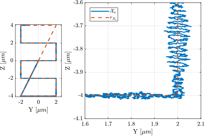
Figure 77: Measured position $X_{n}$ and reference signal $r_{X_{n}}$ in the Y-Z plane - Zoom on a change of direction

Important

It is clear from Figure 77 that the position of the nano-hexapod effectively tracks to reference signal. However, oscillations with amplitudes as large as 50nm can be observe.

It turns out that the frequency of these oscillations is 100Hz which is corresponding to the crossover frequency of the High Authority Control loop. This clearly indicates poor stability margins. In the next section, the controller is re-designed to improve the stability margins.

3.2.4. Controller with increased stability margins

The High Authority Controller is re-designed in order to improve the stability margins.

Copy
%% Lead
a  = 5;  % Amount of phase lead / width of the phase lead / high frequency gain
wc = 2*pi*110; % Frequency with the maximum phase lead [rad/s]

H_lead = (1 + s/(wc/sqrt(a)))/(1 + s/(wc*sqrt(a)));

%% Low Pass Filter
H_lpf = 1/(1 + s/2/pi/300);

%% Notch
gm = 0.02;
xi = 0.5;
wn = 2*pi*700;

H_notch = (s^2 + 2*gm*xi*wn*s + wn^2)/(s^2 + 2*xi*wn*s + wn^2);

%% HAC Controller
Khac_iff_struts = -2.2e4 * ... % Gain
            H_lead * ...       % Lead
            H_lpf * ...        % Lead
            H_notch * ...      % Notch
            (2*pi*100/s) * ... % Integrator
            eye(6);            % 6x6 Diagonal

The bode plot of the new loop gain is shown in Figure 78.

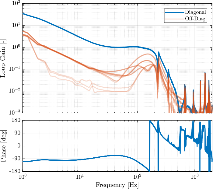
Figure 78: Loop Gain for the updated decentralized HAC controller

This new controller is implemented experimentally and several tracking tests are performed.

Copy
%% Load Measurements
load('hac_iff_more_lead_nass_scan.mat', 't', 'de')

The pose of the top platform is estimated from the encoder position using the Jacobian matrix.

Copy
%% Compute the pose of the top platform
load('jacobian.mat', 'J');
Xe = [inv(J)*de']';

The measured motion as well as the trajectory are shown in Figure 79.

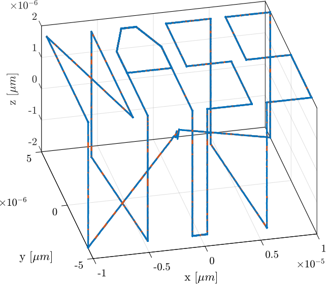
Figure 79: Measured position $X_{n}$ and reference signal $r_{X_{n}}$ for the “NASS” trajectory

The trajectory and measured motion are also shown in the X-Y plane in Figure 80.

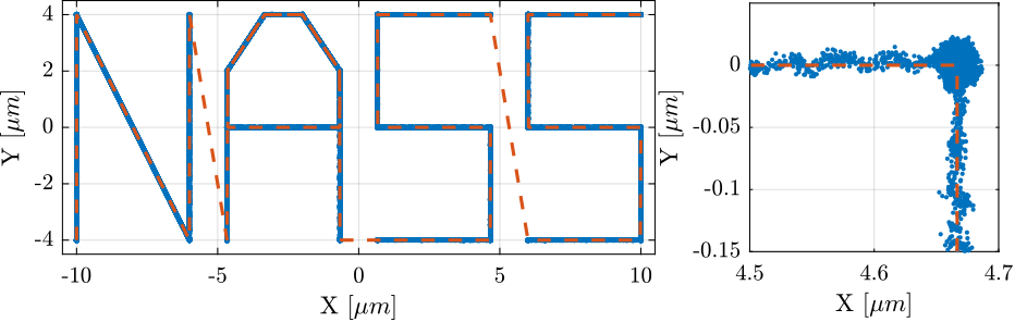
Figure 80: Reference path and measured motion in the X-Y plane

The orientation errors during all the scans are shown in Figure 81.

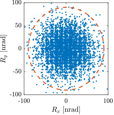
Figure 81: Orientation errors during the scan

Important

Using the updated High Authority Controller, the nano-hexapod can follow trajectories with high accuracy (the position errors are in the order of 50nm peak to peak, and the orientation errors 300nrad peak to peak).

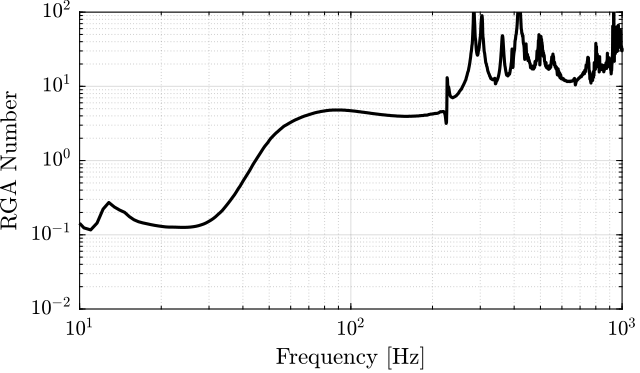
3.3. Interaction Analysis and Decoupling

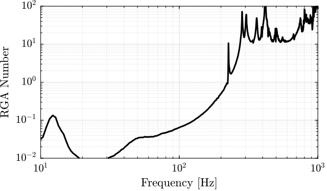
In this section, the interaction in the identified plant is estimated using the Relative Gain Array (RGA) (Skogestad and Postlethwaite 2007, 3.4).

Then, several decoupling strategies are compared for the nano-hexapod.

The RGA Matrix is defined as follow:

\begin{matrix} (2) & RGA (G (f)) = G (f) \times (G (f)^{- 1})^{T} \end{matrix}

Then, the RGA number is defined:

\begin{matrix} (3) & RGA-num (f) = ‖ I - RGA(G(f)) ‖_{sum} \end{matrix}

In this section, the plant with 2 added mass is studied.

3.3.1. Parameters

Copy
wc = 100; % Wanted crossover frequency [Hz]
[~, i_wc] = min(abs(frf_iff.f - wc)); % Indice corresponding to wc

Copy
%% Plant to be decoupled
frf_coupled = frf_iff.G_dL{2};
G_coupled = sim_iff.G_dL{2};

3.3.2. No Decoupling (Decentralized)

Figure 82: Block diagram representing the plant.

Figure 83: Bode Plot of the decentralized plant (diagonal and off-diagonal terms)

Figure 84: RGA number for the decentralized plant

3.3.3. Static Decoupling

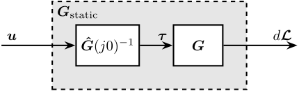
Figure 85: Decoupling using the inverse of the DC gain of the plant

The DC gain is evaluated from the model as be have bad low frequency identification.

-62011.5	3910.6	4299.3	660.7	-4016.5	-4373.6
3914.4	-61991.2	-4356.8	-4019.2	640.2	4281.6
-4020.0	-4370.5	-62004.5	3914.6	4295.8	653.8
660.9	4292.4	3903.3	-62012.2	-4366.5	-4008.9
4302.8	655.6	-4025.8	-4377.8	-62006.0	3919.7
-4377.9	-4013.2	668.6	4303.7	3906.8	-62019.3

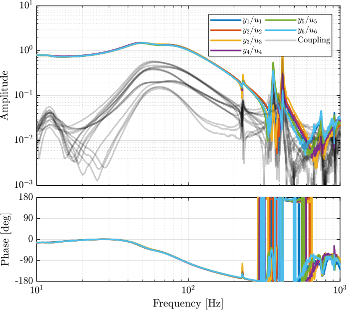
Figure 86: Bode Plot of the static decoupled plant

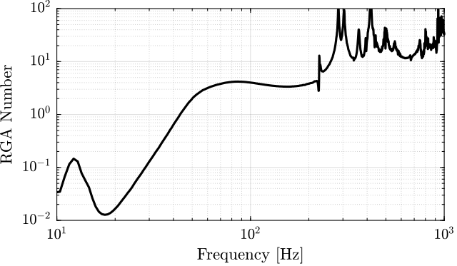
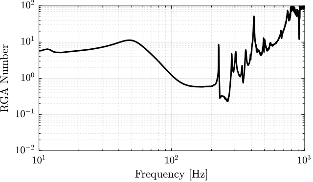
Figure 87: RGA number for the statically decoupled plant

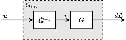
3.3.4. Decoupling at the Crossover

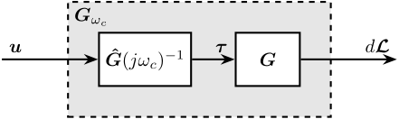
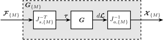
Figure 88: Decoupling using the inverse of a dynamical model $\hat{G}$ of the plant dynamics $G$

67229.8	3769.3	-13704.6	-23084.8	-6318.2	23378.7
3486.2	67708.9	23220.0	-6314.5	-22699.8	-14060.6
-5731.7	22471.7	66701.4	3070.2	-13205.6	-21944.6
-23305.5	-14542.6	2743.2	70097.6	24846.8	-5295.0
-14882.9	-22957.8	-5344.4	25786.2	70484.6	2979.9
24353.3	-5195.2	-22449.0	-14459.2	2203.6	69484.2

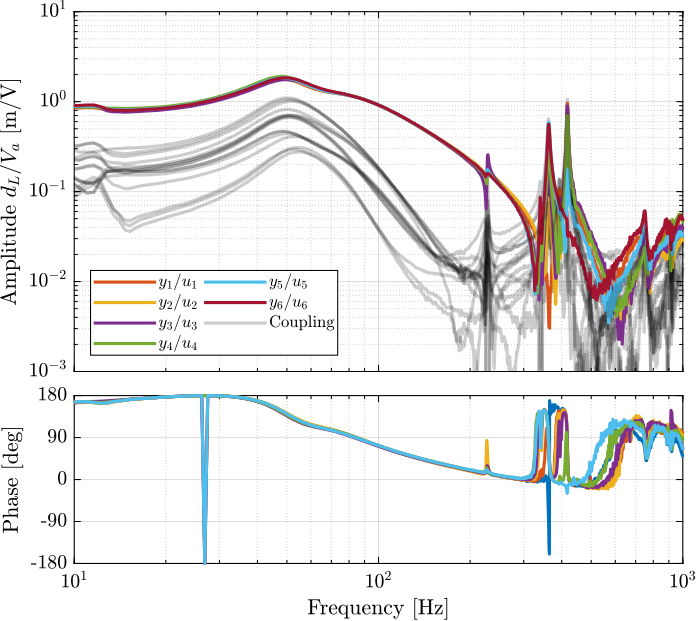
Figure 89: Bode Plot of the plant decoupled at the crossover

Copy
%% Compute RGA Matrix
RGA_wc = zeros(size(frf_coupled));
for i = 1:length(frf_iff.f)
    RGA_wc(i,:,:) = squeeze(G_dL_wc(i,:,:)).*inv(squeeze(G_dL_wc(i,:,:))).';
end

%% Compute RGA-number
RGA_wc_sum = zeros(size(RGA_wc, 1), 1);
for i = 1:size(RGA_wc, 1)
    RGA_wc_sum(i) = sum(sum(abs(eye(6) - squeeze(RGA_wc(i,:,:)))));
end

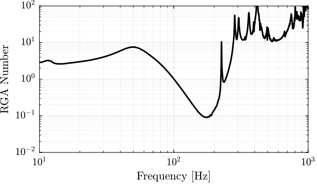
Figure 90: RGA number for the plant decoupled at the crossover

3.3.5. SVD Decoupling

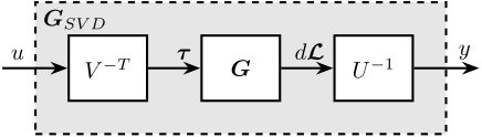
Figure 91: Decoupling using the Singular Value Decomposition

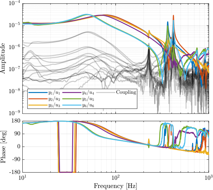
Figure 92: Bode Plot of the plant decoupled using the Singular Value Decomposition

Copy
%% Compute the RGA matrix for the SVD decoupled plant
RGA_svd = zeros(size(frf_coupled));
for i = 1:length(frf_iff.f)
    RGA_svd(i,:,:) = squeeze(G_dL_svd(i,:,:)).*inv(squeeze(G_dL_svd(i,:,:))).';
end

%% Compute the RGA-number
RGA_svd_sum = zeros(size(RGA_svd, 1), 1);
for i = 1:length(frf_iff.f)
    RGA_svd_sum(i) = sum(sum(abs(eye(6) - squeeze(RGA_svd(i,:,:)))));
end

Copy
%% RGA Number for the SVD decoupled plant
figure;
plot(frf_iff.f, RGA_svd_sum, 'k-');
set(gca, 'XScale', 'log'); set(gca, 'YScale', 'log');
xlabel('Frequency [Hz]'); ylabel('RGA Number');
xlim([10, 1e3]); ylim([1e-2, 1e2]);

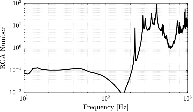
Figure 93: RGA number for the plant decoupled using the SVD

3.3.6. Dynamic decoupling

Figure 94: Decoupling using the inverse of a dynamical model $\hat{G}$ of the plant dynamics $G$

Figure 95: Bode Plot of the dynamically decoupled plant

Figure 96: RGA number for the dynamically decoupled plant

3.3.7. Jacobian Decoupling - Center of Stiffness

Figure 97: Decoupling using Jacobian matrices evaluated at the Center of Stiffness

Figure 98: Bode Plot of the plant decoupled using the Jacobian evaluated at the “center of stiffness”

Figure 99: RGA number for the plant decoupled using the Jacobian evaluted at the Center of Stiffness

3.3.8. Jacobian Decoupling - Center of Mass

Figure 100: Decoupling using Jacobian matrices evaluated at the Center of Mass

Figure 101: Bode Plot of the plant decoupled using the Jacobian evaluated at the Center of Mass

Figure 102: RGA number for the plant decoupled using the Jacobian evaluted at the Center of Mass

3.3.9. Decoupling Comparison

Let’s now compare all of the decoupling methods (Figure 103).

Important

From Figure 103, the following remarks are made:

Decentralized plant: well decoupled below suspension modes
Static inversion: similar to the decentralized plant as the decentralized plant has already a good decoupling at low frequency
Crossover inversion: the decoupling is improved around the crossover frequency as compared to the decentralized plant. However, the decoupling is increased at lower frequency.
SVD decoupling: Very good decoupling up to 235Hz. Especially between 100Hz and 200Hz.
Dynamic Inversion: the plant is very well decoupled at frequencies where the model is accurate (below 235Hz where flexible modes are not modelled).
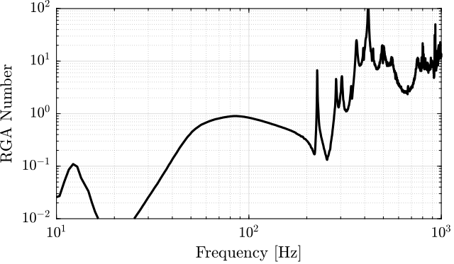
Jacobian - Stiffness: good decoupling at low frequency. The decoupling increases at the frequency of the suspension modes, but is acceptable up to the strut flexible modes (235Hz).
Jacobian - Mass: bad decoupling at low frequency. Better decoupling above the frequency of the suspension modes, and acceptable decoupling up to the strut flexible modes (235Hz).

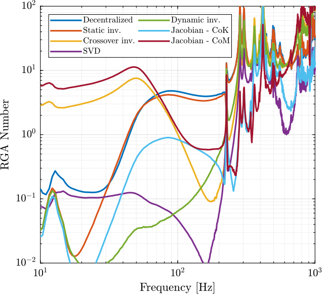
Figure 103: Comparison of the obtained RGA-numbers for all the decoupling methods

3.3.10. Decoupling Robustness

Let’s now see how the decoupling is changing when changing the payload’s mass.

Copyfrf_new = frf_iff.G_dL{3};

The obtained RGA-numbers are shown in Figure 104.

Important

From Figure 104:

The decoupling using the Jacobian evaluated at the “center of stiffness” seems to give the most robust results.

Figure 104: Change of the RGA-number with a change of the payload. Indication of the robustness of the inversion method.

3.3.11. Conclusion

Important

Several decoupling methods can be used:

SVD
Inverse
Jacobian (CoK)

Table 3: Summary of the interaction analysis and different decoupling strategies
Method	RGA	Diag Plant	Robustness
Decentralized	--	Equal	++
Static dec.	--	Equal	++
Crossover dec.	-	Equal	0
SVD	++	Diff	+
Dynamic dec.	++	Unity, equal	-
Jacobian - CoK	+	Diff	++
Jacobian - CoM	0	Diff	+

3.4. Robust High Authority Controller

In this section we wish to develop a robust High Authority Controller (HAC) that is working for all payloads.

(Indri and Oboe 2020)

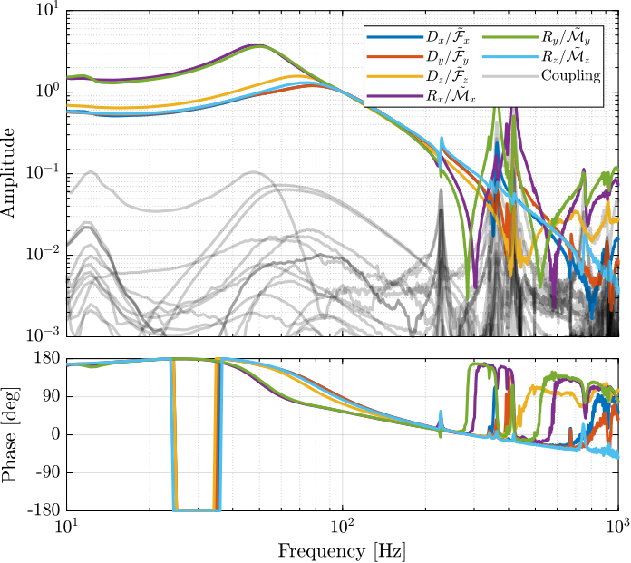
3.4.1. Using Jacobian evaluated at the center of stiffness

3.4.1.1. Decoupled Plant

Copy
G_nom = frf_iff.G_dL{2}; % Nominal Plant

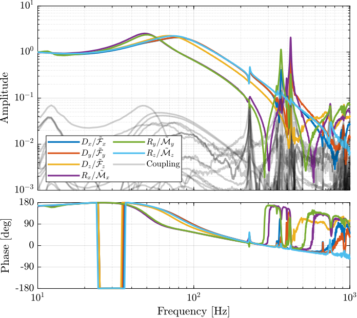
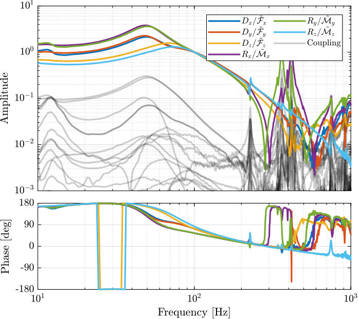
Figure 105: Bode plot of the decoupled plant using the Jacobian evaluated at the Center of Stiffness

3.4.1.2. SISO Controller Design

As the diagonal elements of the plant are not equal, several SISO controllers are designed and then combined to form a diagonal controller. All the diagonal terms of the controller consists of:

A double integrator to have high gain at low frequency
A lead around the crossover frequency to increase stability margins
Two second order low pass filters above the crossover frequency to increase the robustness to high frequency modes

3.4.1.3. Obtained Loop Gain

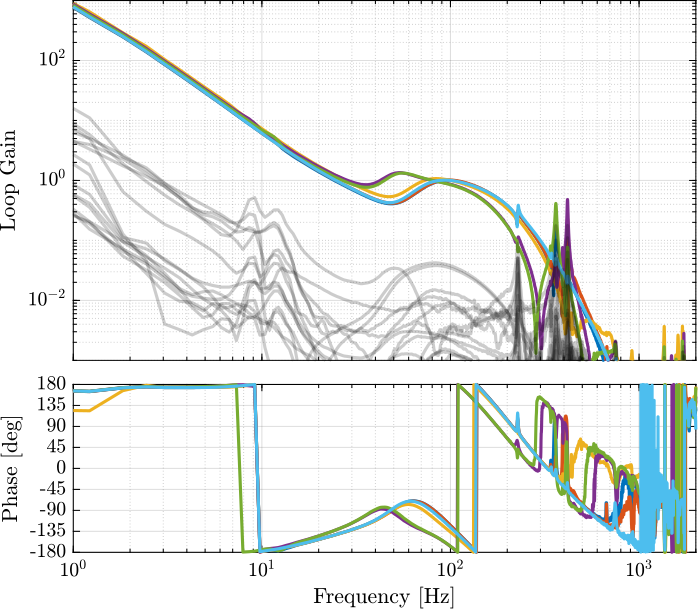
Figure 106: Bode plot of the Loop Gain when using the Jacobian evaluated at the Center of Stiffness to decouple the system

Copy
%% Controller to be implemented
Kd = inv(J_cok')*input_normalize*ss(Kd_diag)*inv(Js_cok);

3.4.1.4. Verification of the Stability

Now the stability of the feedback loop is verified using the generalized Nyquist criteria.

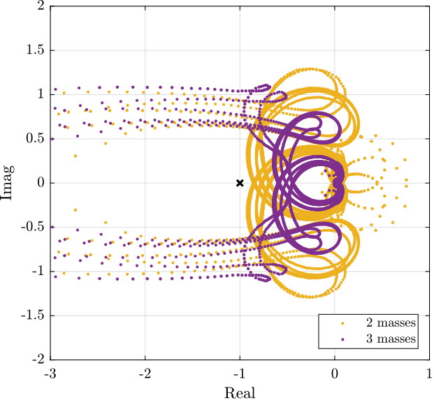
Figure 107: Loci of $L (j ω)$ in the complex plane.

3.4.1.5. Save for further analysis

Copy
save('mat/Khac_iff_struts_jacobian_cok.mat', 'Kd')

3.4.2. Using Singular Value Decomposition

3.4.2.1. Decoupled Plant

Copy
G_nom = frf_iff.G_dL{2}; % Nominal Plant

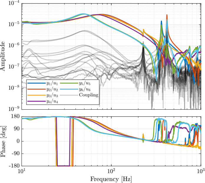
Figure 108: Bode plot of the decoupled plant using the SVD

3.4.2.2. Controller Design

3.4.2.3. Loop Gain

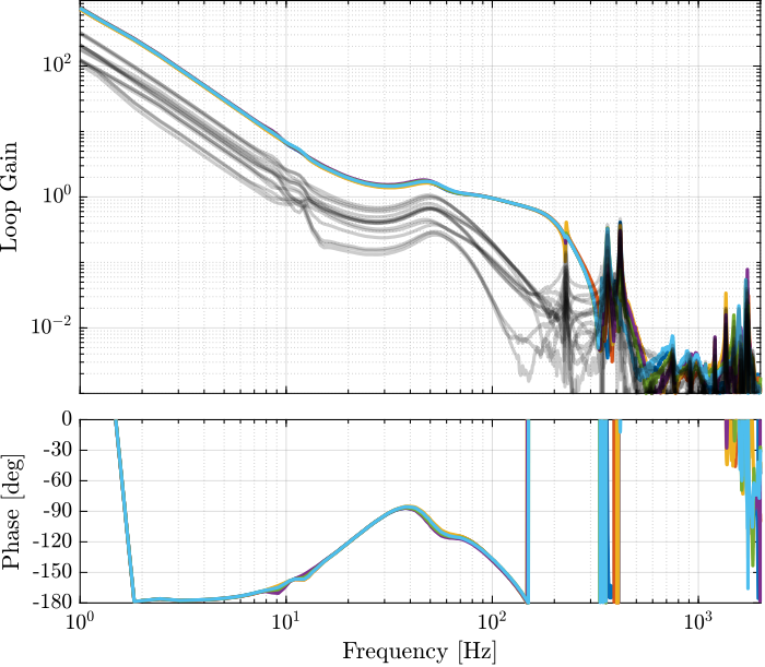
Figure 109: Bode plot of Loop Gain when using the SVD

3.4.2.4. Stability Verification

Copy
%% Compute the Eigenvalues of the loop gain
Ldet = zeros(3, 6, length(frf_iff.f));

for i = 1:3
    Lmimo = pagemtimes(permute(frf_iff.G_dL{i}, [2,3,1]),squeeze(freqresp(Kd, frf_iff.f, 'Hz')));
    for i_f = 2:length(frf_iff.f)
        Ldet(i,:, i_f) = eig(squeeze(Lmimo(:,:,i_f)));
    end
end

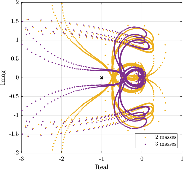
Figure 110: Locis of $L (j ω)$ in the complex plane.

3.4.2.5. Save for further analysis

Copy
save('mat/Khac_iff_struts_svd.mat', 'Kd')

4. Functions

4.1. `generateXYZTrajectory`

Function description

Copy
function [ref] = generateXYZTrajectory(args)
% generateXYZTrajectory -
%
% Syntax: [ref] = generateXYZTrajectory(args)
%
% Inputs:
%    - args
%
% Outputs:
%    - ref - Reference Signal

Optional Parameters

Copyarguments
    args.points double {mustBeNumeric} = zeros(2, 3) % [m]

    args.ti    (1,1) double {mustBeNumeric, mustBeNonnegative} = 1 % Time to go to first point and after last point [s]
    args.tw    (1,1) double {mustBeNumeric, mustBeNonnegative} = 0.5 % Time wait between each point [s]
    args.tm    (1,1) double {mustBeNumeric, mustBeNonnegative} = 1 % Motion time between points [s]

    args.Ts    (1,1) double {mustBeNumeric, mustBePositive} = 1e-3 % Sampling Time [s]
end

Initialize Time Vectors

Copy
time_i = 0:args.Ts:args.ti;
time_w = 0:args.Ts:args.tw;
time_m = 0:args.Ts:args.tm;

XYZ Trajectory

Copy
% Go to initial position
xyz = (args.points(1,:))'*(time_i/args.ti);

% Wait
xyz = [xyz, xyz(:,end).*ones(size(time_w))];

% Scans
for i = 2:size(args.points, 1)
    % Go to next point
    xyz = [xyz, xyz(:,end) + (args.points(i,:)' - xyz(:,end))*(time_m/args.tm)];
    % Wait a litle bit
    xyz = [xyz, xyz(:,end).*ones(size(time_w))];
end

% End motion
xyz = [xyz, xyz(:,end) - xyz(:,end)*(time_i/args.ti)];

Reference Signal

Copy
t = 0:args.Ts:args.Ts*(length(xyz) - 1);

Copyref = zeros(length(xyz), 7);

ref(:, 1) = t;
ref(:, 2:4) = xyz';

4.2. `generateYZScanTrajectory`

Function description

Copy
function [ref] = generateYZScanTrajectory(args)
% generateYZScanTrajectory -
%
% Syntax: [ref] = generateYZScanTrajectory(args)
%
% Inputs:
%    - args
%
% Outputs:
%    - ref - Reference Signal

Optional Parameters

Copyarguments
    args.y_tot (1,1) double {mustBeNumeric, mustBePositive} = 10e-6 % [m]
    args.z_tot (1,1) double {mustBeNumeric, mustBePositive} = 10e-6 % [m]

    args.n     (1,1) double {mustBeInteger, mustBePositive} = 10 % [-]

    args.Ts    (1,1) double {mustBeNumeric, mustBePositive} = 1e-4 % [s]

    args.ti    (1,1) double {mustBeNumeric, mustBeNonnegative} = 1 % [s]
    args.tw    (1,1) double {mustBeNumeric, mustBeNonnegative} = 1 % [s]
    args.ty    (1,1) double {mustBeNumeric, mustBeNonnegative} = 1 % [s]
    args.tz    (1,1) double {mustBeNumeric, mustBeNonnegative} = 1 % [s]
end

Initialize Time Vectors

Copy
time_i = 0:args.Ts:args.ti;
time_w = 0:args.Ts:args.tw;
time_y = 0:args.Ts:args.ty;
time_z = 0:args.Ts:args.tz;

Y and Z vectors

Copy
% Go to initial position
y = (time_i/args.ti)*(args.y_tot/2);

% Wait
y = [y, y(end)*ones(size(time_w))];

% Scans
for i = 1:args.n
    if mod(i,2) == 0
        y = [y, -(args.y_tot/2) + (time_y/args.ty)*args.y_tot];
    else
        y = [y,  (args.y_tot/2) - (time_y/args.ty)*args.y_tot];
    end

    if i < args.n
        y = [y, y(end)*ones(size(time_z))];
    end
end

% Wait a litle bit
y = [y, y(end)*ones(size(time_w))];

% End motion
y = [y, y(end) - y(end)*time_i/args.ti];

Copy
% Go to initial position
z = (time_i/args.ti)*(args.z_tot/2);

% Wait
z = [z, z(end)*ones(size(time_w))];

% Scans
for i = 1:args.n
    z = [z, z(end)*ones(size(time_y))];

    if i < args.n
        z = [z, z(end) - (time_z/args.tz)*args.z_tot/(args.n-1)];
    end
end

% Wait a litle bit
z = [z, z(end)*ones(size(time_w))];

% End motion
z = [z, z(end) - z(end)*time_i/args.ti];

Reference Signal

Copy
t = 0:args.Ts:args.Ts*(length(y) - 1);

Copyref = zeros(length(y), 7);

ref(:, 1) = t;
ref(:, 3) = y;
ref(:, 4) = z;

4.3. `generateSpiralAngleTrajectory`

Function description

Copy
function [ref] = generateSpiralAngleTrajectory(args)
% generateSpiralAngleTrajectory -
%
% Syntax: [ref] = generateSpiralAngleTrajectory(args)
%
% Inputs:
%    - args
%
% Outputs:
%    - ref - Reference Signal

Optional Parameters

Copyarguments
    args.R_tot  (1,1) double {mustBeNumeric, mustBePositive} = 10e-6 % [rad]
    args.n_turn (1,1) double {mustBeInteger, mustBePositive} = 5 % [-]
    args.Ts     (1,1) double {mustBeNumeric, mustBePositive} = 1e-3 % [s]
    args.t_turn (1,1) double {mustBeNumeric, mustBePositive} = 1 % [s]
    args.t_end  (1,1) double {mustBeNumeric, mustBePositive} = 1 % [s]
end

Initialize Time Vectors

Copy
time_s = 0:args.Ts:args.n_turn*args.t_turn;
time_e = 0:args.Ts:args.t_end;

Rx and Ry vectors

Copy
Rx = sin(2*pi*time_s/args.t_turn).*(args.R_tot*time_s/(args.n_turn*args.t_turn));
Ry = cos(2*pi*time_s/args.t_turn).*(args.R_tot*time_s/(args.n_turn*args.t_turn));

Copy
Rx = [Rx, 0*time_e];
Ry = [Ry, Ry(end) - Ry(end)*time_e/args.t_end];

Reference Signal

Copy
t = 0:args.Ts:args.Ts*(length(Rx) - 1);

Copyref = zeros(length(Rx), 7);

ref(:, 1) = t;
ref(:, 5) = Rx;
ref(:, 6) = Ry;

4.4. `getTransformationMatrixAcc`

Function description

Copy
function [M] = getTransformationMatrixAcc(Opm, Osm)
% getTransformationMatrixAcc -
%
% Syntax: [M] = getTransformationMatrixAcc(Opm, Osm)
%
% Inputs:
%    - Opm - Nx3 (N = number of accelerometer measurements) X,Y,Z position of accelerometers
%    - Opm - Nx3 (N = number of accelerometer measurements) Unit vectors representing the accelerometer orientation
%
% Outputs:
%    - M - Transformation Matrix

Transformation matrix from motion of the solid body to accelerometer measurements

Let’s try to estimate the x-y-z acceleration of any point of the solid body from the acceleration/angular acceleration of the solid body expressed in ${O}$ . For any point $p_{i}$ of the solid body (corresponding to an accelerometer), we can write:

\begin{matrix} (4) & [\begin{matrix} a_{i, x} \\ a_{i, y} \\ a_{i, z} \end{matrix}] = [\begin{matrix} {\dot{v}}_{x} \\ {\dot{v}}_{y} \\ {\dot{v}}_{z} \end{matrix}] + p_{i} \times [\begin{matrix} {\dot{ω}}_{x} \\ {\dot{ω}}_{y} \\ {\dot{ω}}_{z} \end{matrix}] \end{matrix}

We can write the cross product as a matrix product using the skew-symmetric transformation:

\begin{matrix} (5) & [\begin{matrix} a_{i, x} \\ a_{i, y} \\ a_{i, z} \end{matrix}] = [\begin{matrix} {\dot{v}}_{x} \\ {\dot{v}}_{y} \\ {\dot{v}}_{z} \end{matrix}] + \underset{P_{i, [\times]}}{\underset{⏟}{[\begin{matrix} 0 & p_{i, z} & - p_{i, y} \\ - p_{i, z} & 0 & p_{i, x} \\ p_{i, y} & - p_{i, x} & 0 \end{matrix}]}} \cdot [\begin{matrix} {\dot{ω}}_{x} \\ {\dot{ω}}_{y} \\ {\dot{ω}}_{z} \end{matrix}] \end{matrix}

If we now want to know the (scalar) acceleration $a_{i}$ of the point $p_{i}$ in the direction of the accelerometer direction ${\hat{s}}_{i}$ , we can just project the 3d acceleration on ${\hat{s}}_{i}$ :

\begin{matrix} (6) & a_{i} = {\hat{s}}_{i}^{T} \cdot [\begin{matrix} a_{i, x} \\ a_{i, y} \\ a_{i, z} \end{matrix}] = {\hat{s}}_{i}^{T} \cdot [\begin{matrix} {\dot{v}}_{x} \\ {\dot{v}}_{y} \\ {\dot{v}}_{z} \end{matrix}] + ({\hat{s}}_{i}^{T} \cdot P_{i, [\times]}) \cdot [\begin{matrix} {\dot{ω}}_{x} \\ {\dot{ω}}_{y} \\ {\dot{ω}}_{z} \end{matrix}] \end{matrix}

Which is equivalent as a simple vector multiplication:

\begin{matrix} (7) & a_{i} = [\begin{matrix} {\hat{s}}_{i}^{T} & {\hat{s}}_{i}^{T} \cdot P_{i, [\times]} \end{matrix}] [\begin{matrix} {\dot{v}}_{x} \\ {\dot{v}}_{y} \\ {\dot{v}}_{z} \\ {\dot{ω}}_{x} \\ {\dot{ω}}_{y} \\ {\dot{ω}}_{z} \end{matrix}] = [\begin{matrix} {\hat{s}}_{i}^{T} & {\hat{s}}_{i}^{T} \cdot P_{i, [\times]} \end{matrix}]^{O} \vec{x} \end{matrix}

And finally we can combine the 6 (line) vectors for the 6 accelerometers to write that in a matrix form. We obtain Eq. $(8)$ .

Important

The transformation from solid body acceleration $^{O} \vec{x}$ from sensor measured acceleration $\vec{a}$ is:

\begin{matrix} (8) & \vec{a} = \underset{M}{\underset{⏟}{[\begin{matrix} {\hat{s}}_{1}^{T} & {\hat{s}}_{1}^{T} \cdot P_{1, [\times]} \\ ⋮ & ⋮ \\ {\hat{s}}_{6}^{T} & {\hat{s}}_{6}^{T} \cdot P_{6, [\times]} \end{matrix}]}}^{O} \vec{x} \end{matrix}

with ${\hat{s}}_{i}$ the unit vector representing the measured direction of the i’th accelerometer expressed in frame ${O}$ and $P_{i, [\times]}$ the skew-symmetric matrix representing the cross product of the position of the i’th accelerometer expressed in frame ${O}$ .

Let’s define such matrix using matlab:

CopyM = zeros(length(Opm), 6);

for i = 1:length(Opm)
    Ri = [0,         Opm(3,i), -Opm(2,i);
         -Opm(3,i),  0,         Opm(1,i);
          Opm(2,i), -Opm(1,i),  0];
    M(i, 1:3) = Osm(:,i)';
    M(i, 4:6) = Osm(:,i)'*Ri;
end

Copy
end

4.5. `getJacobianNanoHexapod`

Function description

Copy
function [J] = getJacobianNanoHexapod(Hbm)
% getJacobianNanoHexapod -
%
% Syntax: [J] = getJacobianNanoHexapod(Hbm)
%
% Inputs:
%    - Hbm - Height of {B} w.r.t. {M} [m]
%
% Outputs:
%    - J - Jacobian Matrix

Transformation matrix from motion of the solid body to accelerometer measurements

Copy
Fa = [[-86.05,  -74.78, 22.49],
      [ 86.05,  -74.78, 22.49],
      [ 107.79, -37.13, 22.49],
      [ 21.74,  111.91, 22.49],
      [-21.74,  111.91, 22.49],
      [-107.79, -37.13, 22.49]]'*1e-3; % Ai w.r.t. {F} [m]

Mb = [[-28.47, -106.25, -22.50],
      [ 28.47, -106.25, -22.50],
      [ 106.25, 28.47,  -22.50],
      [ 77.78,  77.78,  -22.50],
      [-77.78,  77.78,  -22.50],
      [-106.25, 28.47,  -22.50]]'*1e-3; % Bi w.r.t. {M} [m]

H = 95e-3; % Stewart platform height [m]
Fb = Mb + [0; 0; H]; % Bi w.r.t. {F} [m]

si = Fb - Fa;
si = si./vecnorm(si); % Normalize

Bb = Mb - [0; 0; Hbm];

J = [si', cross(Bb, si)'];

Bibliography

Indri, Marina, and Roberto Oboe. 2020. Mechatronics and Robotics: New Trends and Challenges. CRC Press.

Skogestad, Sigurd, and Ian Postlethwaite. 2007. Multivariable Feedback Control: Analysis and Design - Second Edition. John Wiley.

Table of Contents

Nano-Hexapod - Test Bench

Table of ContentsClose

1. Encoders fixed to the Struts - Dynamics

1.1. Identification of the dynamics

1.1.1. Load Measurement Data

1.1.2. Spectral Analysis - Setup

1.1.3. Transfer function from Actuator to Encoder

1.1.4. Transfer function from Actuator to Force Sensor

1.1.5. Save Identified Plants

1.2. Comparison with the Simscape Model

1.2.1. Load measured FRF

1.2.2. Dynamics from Actuator to Force Sensors

1.2.3. Dynamics from Actuator to Encoder

1.2.4. Effect of a change in bending damping of the joints

1.2.5. Effect of a change in damping factor of the APA

1.2.6. Effect of a change in stiffness damping coef of the APA

1.2.7. Effect of a change in mass damping coef of the APA

1.2.8. Using Flexible model

1.2.9. Flexible model + encoders fixed to the plates

1.3. Integral Force Feedback

1.3.1. IFF Control Law and Optimal Gain

1.3.2. Effect of IFF on the plant - Simulations

1.3.3. Effect of IFF on the plant - Experimental Results

1.3.3.1. Load Data

1.3.3.2. Spectral Analysis - Setup

1.3.3.3. DVF Plant

1.3.3.4. Experimental Results - Comparison of the un-damped and fully damped system

1.3.4. Experimental Results - Damped Plant with Optimal gain

1.3.4.1. Load Data

1.3.4.2. Spectral Analysis - Setup

1.3.4.3. DVF Plant

1.3.5. Comparison with the Flexible model

1.3.6. Conclusion

1.4. Modal Analysis

1.4.1. Obtained Mode Shapes

1.4.2. Nano-Hexapod Compliance - Effect of IFF

1.4.3. Comparison with the Simscape Model

1.5. Conclusion

2. Encoders fixed to the plates - Dynamics

2.1. Identification of the dynamics

2.1.1. Data Loading and Spectral Analysis Setup

2.1.2. Transfer function from Actuator to Encoder

2.1.3. Transfer function from Actuator to Force Sensor

2.1.4. Save Identified Plants

2.2. Comparison with the Simscape Model

2.2.1. Identification Setup

2.2.2. Dynamics from Actuator to Force Sensors

2.2.3. Dynamics from Actuator to Encoder

2.2.4. Flexible Top Plate

2.2.5. Conclusion

2.3. Integral Force Feedback

2.3.1. Effect of IFF on the plant - Simscape Model

2.3.2. Effect of IFF on the plant - FRF

2.3.3. Comparison of the measured FRF and the Simscape model

2.3.4. Save Damped Plant

2.4. Effect of Payload mass - Robust IFF

2.4.1. Measured Frequency Response Functions

2.4.1.1. Compute FRF in open-loop

2.4.2. Transfer function from u to dLm

2.4.3. Transfer function from u to τm

2.5. Comparison with the Simscape model

2.5.1. System Identification

2.5.2. Transfer function from u to dLm

2.5.3. Transfer function from u to τm

2.6. Integral Force Feedback Controller

2.6.1. Robust IFF Controller

2.6.2. Estimated Damped Plant from the Simscape model

2.6.3. Compute the identified FRF with IFF

2.6.4. Comparison of the measured FRF and the Simscape model

2.6.5. Change of coupling with IFF

2.7. Un-Balanced mass

2.7.1. Introduction

2.7.2. Compute the identified FRF with IFF

2.7.3. Effect of an unbalanced payload

2.8. Conclusion

3. Decentralized High Authority Control with Integral Force Feedback

3.1. Reference Tracking - Trajectories

3.1.1. Y-Z Scans

3.1.2. Tilt Scans

2.4.2. Transfer function from $u$ to $d L_{m}$

2.4.3. Transfer function from $u$ to $τ_{m}$

2.5.2. Transfer function from $u$ to $d L_{m}$

2.5.3. Transfer function from $u$ to $τ_{m}$

4.1. `generateXYZTrajectory`

4.2. `generateYZScanTrajectory`

4.3. `generateSpiralAngleTrajectory`

4.4. `getTransformationMatrixAcc`

4.5. `getJacobianNanoHexapod`