Nano-Hexapod Struts - Test Bench
Table of Contents
- 1. Model of the Amplified Piezoelectric Actuator
- 2. First Basic Measurements
- 3. Dynamical measurements - APA
- 4. Test Bench APA300ML - Simscape Model
- 5. Dynamical measurements - Struts
- 6. Test Bench Struts - Simscape Model
- 7. Function
- 7.1.
initializeBotFlexibleJoint- Initialize Flexible Joint - 7.2.
initializeTopFlexibleJoint- Initialize Flexible Joint - 7.3.
initializeAPA- Initialize APA - 7.4.
generateSweepExc: Generate sweep sinus excitation - 7.5.
generateShapedNoise: Generate Shaped Noise excitation - 7.6.
generateSinIncreasingAmpl: Generate Sinus with increasing amplitude
- 7.1.
This report is also available as a pdf.
In this document, a test-bench is used to characterize the struts of the nano-hexapod.
Each strut includes (Figure 1):
- 2 flexible joints at each ends. These flexible joints have been characterized in a separate test bench.
- 1 Amplified Piezoelectric Actuator (APA300ML) (described in Section 1). Two stacks are used as an actuator and one stack as a (force) sensor.
- 1 encoder (Renishaw Vionic) that has been characterized in a separate test bench.
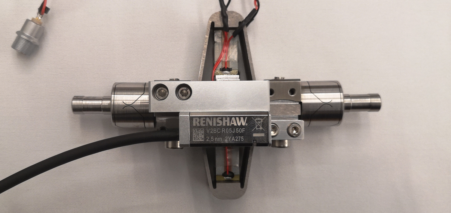
Figure 1: One strut including two flexible joints, an amplified piezoelectric actuator and an encoder
The first goal is to characterize the APA300ML in terms of:
- The, geometric features, electrical capacitance, stroke, hysteresis, spurious resonances. This is performed in Section 2.
- The dynamics from the generated DAC voltage (going to the voltage amplifiers and then applied on the actuator stacks) to the induced displacement, and to the measured voltage by the force sensor stack. Also the “actuator constant” and “sensor constant” are identified. This is done in Section 3.
- Compare the measurements with the Simscape models (2DoF, Super-Element) in order to tuned/validate the models. This is explained in Section 4.
Then the struts are mounted (procedure described here), and are fixed to the same measurement bench. Similarly, the goals are to:
- Section 5: Identify the dynamics from the generated DAC voltage to:
- the sensors stack generated voltage
- the measured displacement by the encoder
- the measured displacement by the interferometer (representing encoders that would be fixed to the nano-hexapod’s plates instead of the struts)
- Section 6: Compare the measurements with the Simscape model of the struts and tune the models
The final goal of the work presented in this document is to have an accurate Simscape model of the struts that can then be included in the Simscape model of the nano-hexapod.
1 Model of the Amplified Piezoelectric Actuator
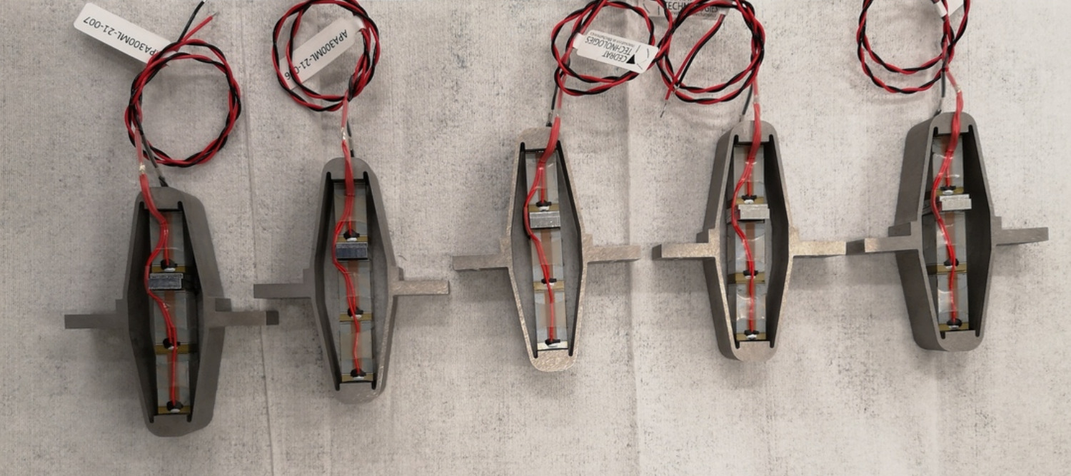
The Amplified Piezoelectric Actuator (APA) used is the APA300ML from Cedrat technologies (Figure 2).
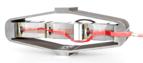
Figure 2: Picture of the APA300ML
Two simscape models of the APA300ML are developed:
- Section 1.1: a simple 2 degrees of freedom (DoF) model
- Section 1.2: a “flexible” model using a “super-element” extracted from a Finite Element Model of the APA
For both models, an “actuator constant” and a “sensor constant” are used. These constants are used to link the electrical domain and the mechanical domain. They are described in Section 1.3.
1.1 Two Degrees of Freedom Model
The presented model is based on (Souleille et al. 2018) and represented in Figure 3.
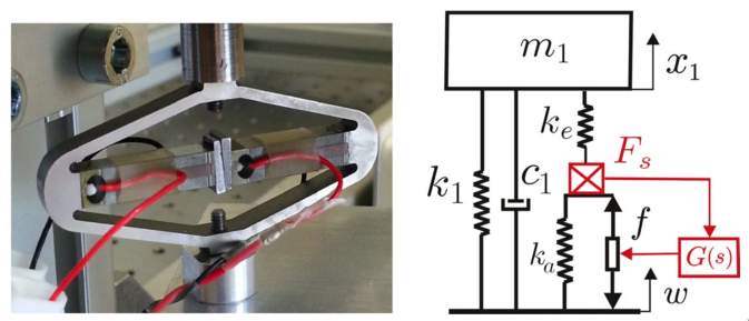
Figure 3: Picture of an APA100M from Cedrat Technologies. Simplified model of a one DoF payload mounted on such isolator
The parameters are described in Table 1.
| Meaning | |
|---|---|
| \(k_e\) | Stiffness used to adjust the pole of the isolator |
| \(k_1\) | Stiffness of the metallic suspension when the stack is removed |
| \(k_a\) | Stiffness of the actuator |
| \(c_1\) | Added viscous damping |
The model is shown again in Figure 4. As will be shown in the next section, such model can be quite accurate in modelling the axial behavior of the APA. However, it does not model the flexibility of the APA in the other directions.
Therefore this model can be useful for quick simulations as it contains a very limited number of states, but when more complex dynamics of the APA is to be modelled, a flexible model will be used.

Figure 4: Schematic of the 2DoF model for the Amplified Piezoelectric Actuator
1.2 Flexible Model
In order to model with high accuracy the behavior of the APA, a flexible model can be used.
The idea is to do a Finite element model of the structure, and to defined “remote points” as shown in Figure 5. Then, on the finite element software, a “super-element” can be extracted which consists of a mass matrix, a stiffness matrix, and the coordinates of the remote points.
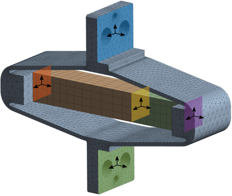
Figure 5: Remote points for the APA300ML (Ansys)
This “super-element” can then be included in the Simscape model as shown in Figure 6. The remotes points are defined as “frames” in Simscape, and the “super-element” can be connected with other Simscape elements (mechanical joints, masses, force actuators, etc..).
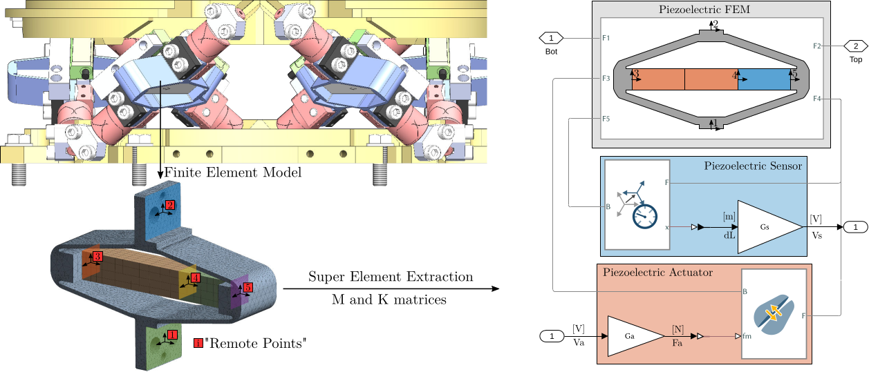
Figure 6: From a finite Element Model (Ansys, bottom left) is extract the mass and stiffness matrices that are then used on Simscape (right)
1.3 Actuator and Sensor constants
On Simscape, we want to model both the actuator stacks and the sensors stack. We therefore need to link the electrical domain (voltages, charges) with the mechanical domain (forces, strain). To do so, we use the “actuator constant” and the “sensor constant”.
Consider a schematic of the Amplified Piezoelectric Actuator in Figure 7.
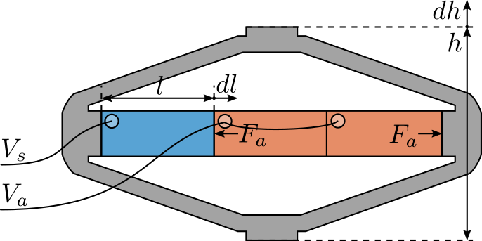
Figure 7: Amplified Piezoelectric Actuator Schematic
A voltage \(V_a\) applied to the actuator stacks will induce an actuator force \(F_a\):
\begin{equation} \boxed{F_a = g_a \cdot V_a} \end{equation}A change of length \(dl\) of the sensor stack will induce a voltage \(V_s\):
\begin{equation} \boxed{V_s = g_s \cdot dl} \end{equation}The block-diagram model of the piezoelectric actuator is then as shown in Figure 8.
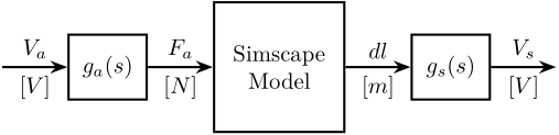
Figure 8: Model of the APA with Simscape/Simulink
The constants \(g_a\) and \(g_s\) will be experimentally estimated.
2 First Basic Measurements
Before using the measurement bench to characterize the APA300ML, first simple measurements are performed:
2.1 Geometrical Measurements
2.1.1 Measurement Setup
The flatness corresponding to the two interface planes are measured as shown in Figure 10.
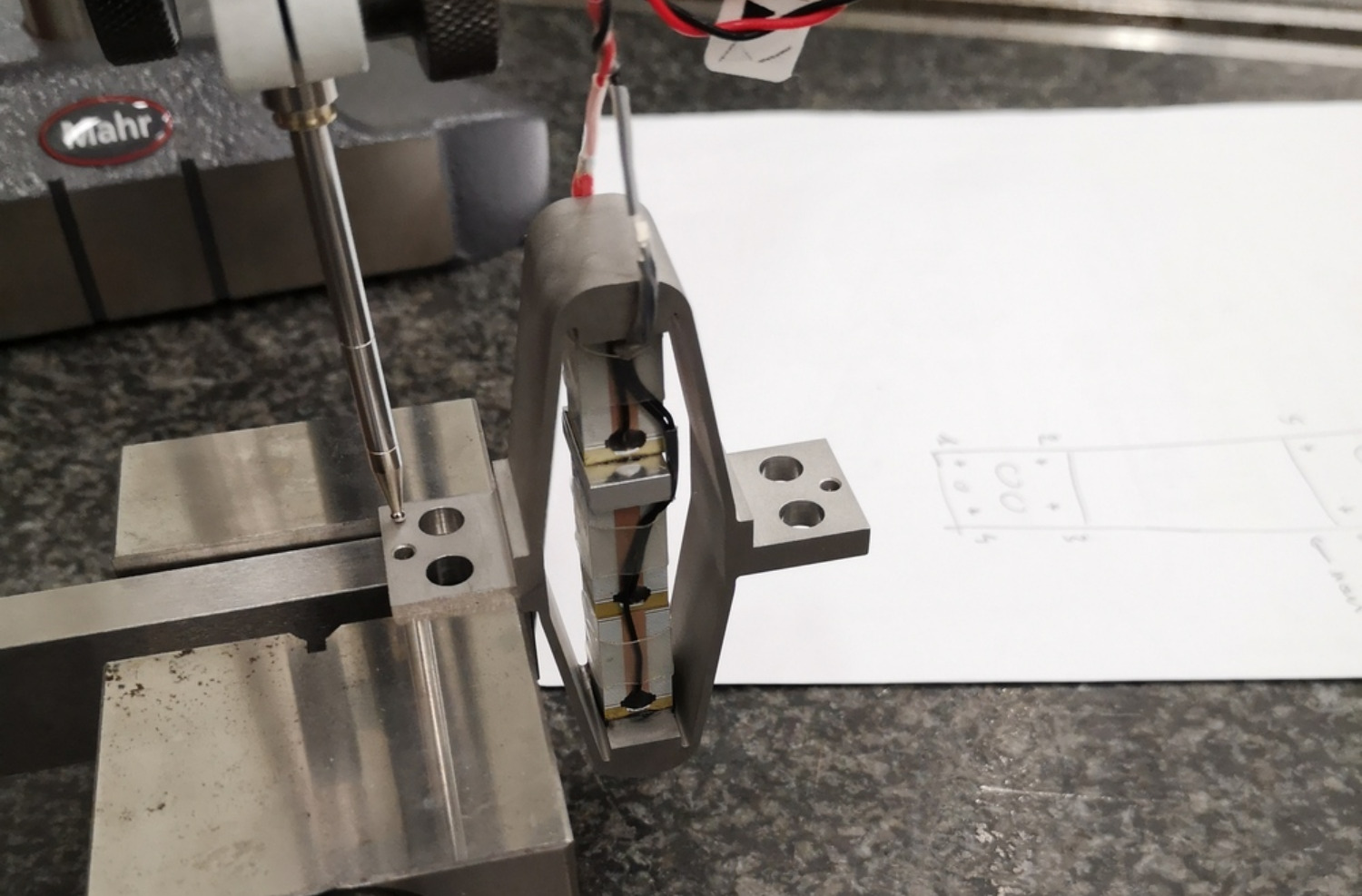
Figure 10: Measurement Setup
2.1.2 Measurement Results
The height (Z) measurements at the 8 locations (4 points by plane) are defined below.
%% Measured height for all the APA at the 8 locations
apa1  = 1e-6*[0, -0.5 , 3.5  , 3.5  , 42   , 45.5, 52.5 , 46];
apa2  = 1e-6*[0, -2.5 , -3   , 0    , -1.5 , 1   , -2   , -4];
apa3  = 1e-6*[0, -1.5 , 15   , 17.5 , 6.5  , 6.5 , 21   , 23];
apa4  = 1e-6*[0, 6.5  , 14.5 , 9    , 16   , 22  , 29.5 , 21];
apa5  = 1e-6*[0, -12.5, 16.5 , 28.5 , -43  , -52 , -22.5, -13.5];
apa6  = 1e-6*[0, -8   , -2   , 5    , -57.5, -62 , -55.5, -52.5];
apa7  = 1e-6*[0, 19.5 , -8   , -29.5, 75   , 97.5, 70   , 48];
apa7b = 1e-6*[0, 9    , -18.5, -30  , 31   , 46.5, 16.5 , 7.5];

apa = {apa1, apa2, apa3, apa4, apa5, apa6, apa7b};
The X/Y Positions of the 8 measurement points are defined below.
%% X-Y positions of the measurements points
W = 20e-3;   % Width [m]
L = 61e-3;   % Length [m]
d = 1e-3;    % Distance from border [m]
l = 15.5e-3; % [m]

pos = [[-L/2 + d;      W/2 - d],
       [-L/2 + l - d;  W/2 - d],
       [-L/2 + l - d; -W/2 + d],
       [-L/2 + d;     -W/2 + d],
       [L/2 - l + d;   W/2 - d],
       [L/2 - d;       W/2 - d],
       [L/2 - d;      -W/2 + d],
       [L/2 - l + d;  -W/2 + d]];
Finally, the flatness is estimated by fitting a plane through the 8 points using the fminsearch command.
%% Using fminsearch to find the best fitting plane
apa_d = zeros(1, 7);
for i = 1:7
    fun = @(x)max(abs(([pos; apa{i}]-[0;0;x(1)])'*([x(2:3);1]/norm([x(2:3);1]))));
    x0 = [0;0;0];
    [x, min_d] = fminsearch(fun,x0);
    apa_d(i) = min_d;
end
The obtained flatness are shown in Table 2.
| Flatness \([\mu m]\) | |
|---|---|
| APA 1 | 8.9 |
| APA 2 | 3.1 |
| APA 3 | 9.1 |
| APA 4 | 3.0 |
| APA 5 | 1.9 |
| APA 6 | 7.1 |
| APA 7 | 18.7 |
The measured flatness of the APA300ML interface planes are within the specifications.
2.2 Electrical Measurements
2.2.1 Measurement Setup
The capacitance of the stacks is measure with the LCR-800 Meter (doc) shown in Figure 11. The excitation frequency is set to be 1kHz.
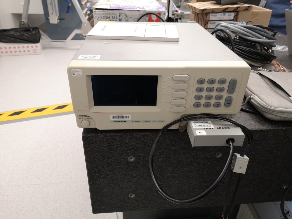
Figure 11: LCR Meter used for the measurements
2.2.2 Measured Capacitance
From the documentation of the APA300ML, the total capacitance of the three stacks should be between \(18\mu F\) and \(26\mu F\) with a nominal capacitance of \(20\mu F\). However, from the documentation of the stack themselves, it can be seen that the capacitance of a single stack should be \(4.4\mu F\). Clearly, the total capacitance of the APA300ML if more than just three times the capacitance of one stack.
Could it be possible that the capacitance of the stacks increase that much when they are pre-stressed?
The measured capacitance of the stacks are summarized in Table 3.
| Sensor Stack | Actuator Stacks | |
|---|---|---|
| APA 1 | 5.10 | 10.03 |
| APA 2 | 4.99 | 9.85 |
| APA 3 | 1.72 | 5.18 |
| APA 4 | 4.94 | 9.82 |
| APA 5 | 4.90 | 9.66 |
| APA 6 | 4.99 | 9.91 |
| APA 7 | 4.85 | 9.85 |
From the measurements (Table 3), the capacitance of one stack is found to be \(\approx 5 \mu F\).
There is clearly a problem with APA300ML number 3 The APA number 3 has ben sent back to Cedrat, and a new APA300ML has been shipped back.
2.3 Stroke measurement
We here wish to estimate the stroke of the APA.
To do so, one side of the APA is fixed, and a displacement probe is located on the other side as shown in Figure 12.
Then, a voltage is applied on either one or two stacks using a DAC and a voltage amplifier.
Here are the documentation of the equipment used for this test bench:
- Voltage Amplifier: PD200 with a gain of 20
- 16bits DAC: IO313 Speedgoat card
- Displacement Probe: Millimar C1216 electronics and Millimar 1318 probe
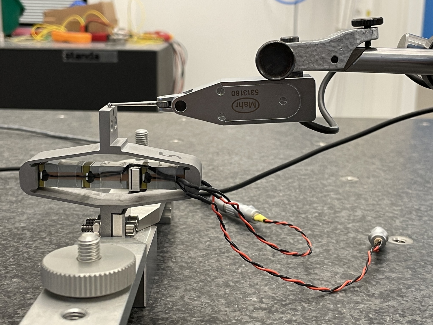
Figure 12: Bench to measured the APA stroke
From the documentation, the nominal stroke of the APA300ML is \(304\,\mu m\).
2.3.1 Voltage applied on one stack
Let’s first look at the relation between the voltage applied to one stack to the displacement of the APA as measured by the displacement probe.
The applied voltage is shown in Figure 13.
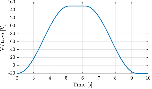
Figure 13: Applied voltage as a function of time
The obtained displacements for all the APA are shown in Figure 14. The displacement is set to zero at initial time when the voltage applied is -20V.
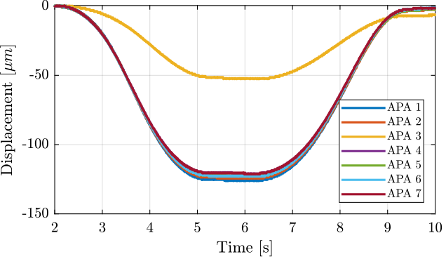
Figure 14: Displacement as a function of time for all the APA300ML (only one stack is used as an actuator)
Finally, the displacement is shown as a function of the applied voltage in Figure 15. We can clearly see that there is a problem with the APA 3. Also, there is a large hysteresis.
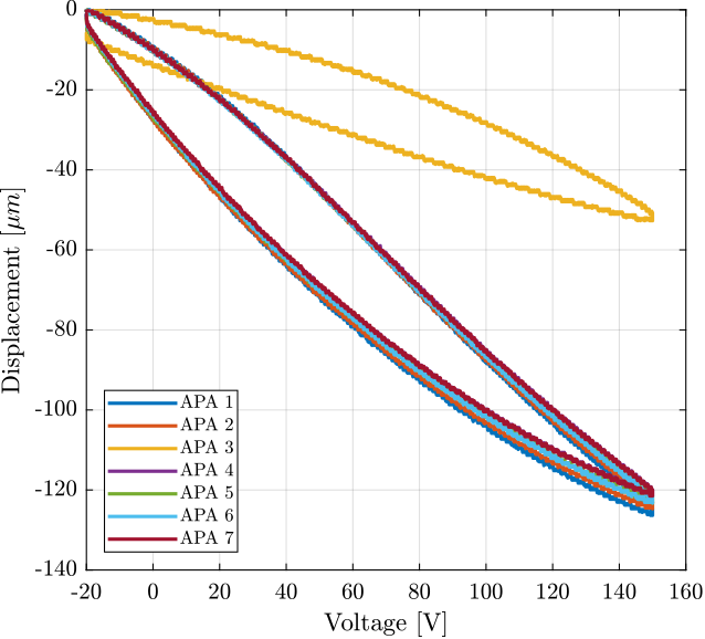
Figure 15: Displacement as a function of the applied voltage (on only one stack)
We can clearly confirm from Figure 15 that there is a problem with the APA number 3.
2.3.2 Voltage applied on two stacks
Now look at the relation between the voltage applied to the two other stacks to the displacement of the APA as measured by the displacement probe.
The obtained displacement is shown in Figure 16. The displacement is set to zero at initial time when the voltage applied is -20V.
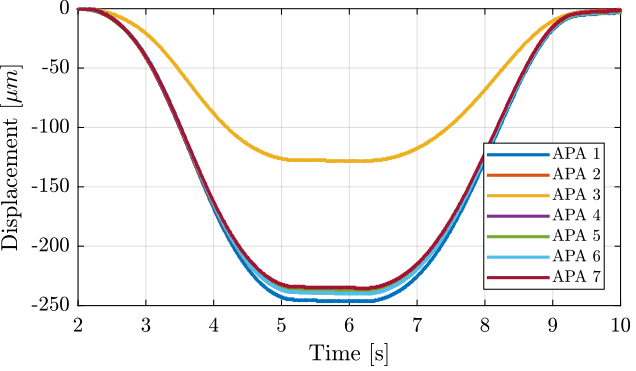
Figure 16: Displacement as a function of time for all the APA300ML (two stacks are used as actuators)
Finally, the displacement is shown as a function of the applied voltage in Figure 17.
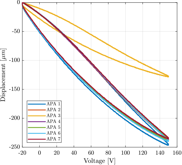
Figure 17: Displacement as a function of the applied voltage on two stacks
2.3.3 Voltage applied on all three stacks
Finally, we can combine the two measurements to estimate the relation between the displacement and the voltage applied to the three stacks (Figure 18).
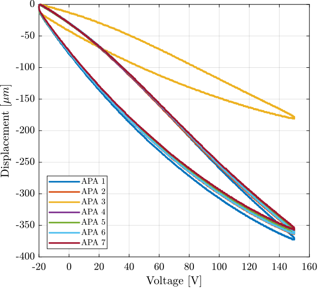
Figure 18: Displacement as a function of the applied voltage on all three stacks
The obtained maximum stroke for all the APA are summarized in Table 4.
| Stroke \([\mu m]\) | |
|---|---|
| APA 1 | 373.2 |
| APA 2 | 365.5 |
| APA 3 | 181.7 |
| APA 4 | 359.7 |
| APA 5 | 361.5 |
| APA 6 | 363.9 |
| APA 7 | 358.4 |
2.3.4 Conclusion
The except from APA 3 that has a problem, all the APA are similar when it comes to stroke and hysteresis. Also, the obtained stroke is more than specified in the documentation. Therefore, only two stacks can be used as an actuator.
2.4 Spurious resonances
2.4.1 Introduction
From a Finite Element Model of the struts, it have been found that three main resonances are foreseen to be problematic for the control of the APA300ML (Figure 19):
- Mode in X-bending at 200Hz
- Mode in Y-bending at 285Hz
- Mode in Z-torsion at 400Hz
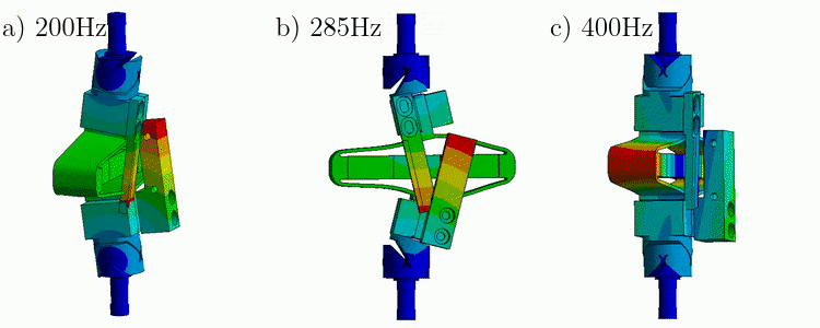
Figure 19: Spurious resonances. a) X-bending mode at 189Hz. b) Y-bending mode at 285Hz. c) Z-torsion mode at 400Hz
These modes are present when flexible joints are fixed to the ends of the APA300ML.
In this section, we try to find the resonance frequency of these modes when one end of the APA is fixed and the other is free.
2.4.2 Measurement Setup
The measurement setup is shown in Figure 20. A Laser vibrometer is measuring the difference of motion between two points. The APA is excited with an instrumented hammer and the transfer function from the hammer to the measured rotation is computed.
The instrumentation used are:
- Laser Doppler Vibrometer Polytec OFV512
- Instrumented hammer

Figure 20: Measurement setup with a Laser Doppler Vibrometer and one instrumental hammer
2.4.3 X-Bending Mode
The vibrometer is setup to measure the X-bending motion is shown in Figure 21. The APA is excited with an instrumented hammer having a solid metallic tip. The impact point is on the back-side of the APA aligned with the top measurement point.
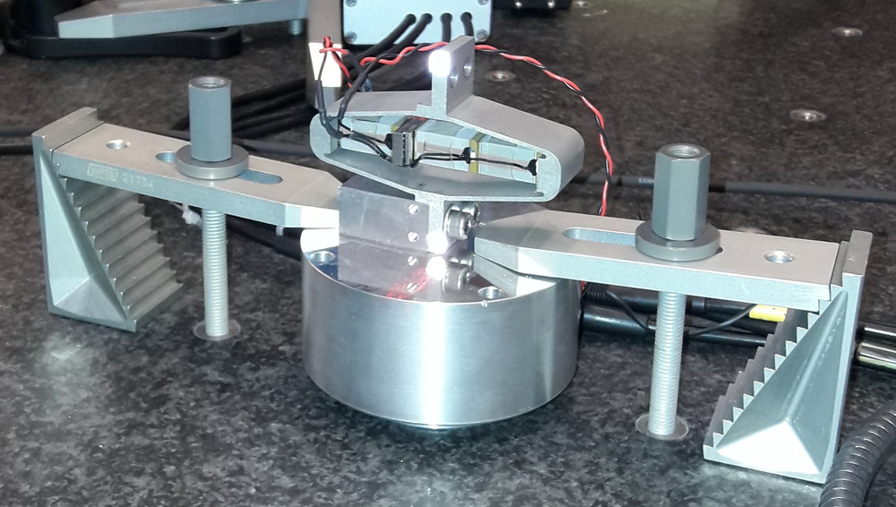
Figure 21: X-Bending measurement setup
The data is loaded.
%% Load Data
bending_X = load('apa300ml_bending_X_top.mat');
The configuration (Sampling time and windows) for tfestimate is done:
%% Spectral Analysis setup
Ts = bending_X.Track1_X_Resolution; % Sampling Time [s]
win = hann(ceil(1/Ts));
The transfer function from the input force to the output “rotation” (difference between the two measured distances).
%% Compute the transfer function from applied force to measured rotation
[G_bending_X, f]  = tfestimate(bending_X.Track1, bending_X.Track2, win, [], [], 1/Ts);
The result is shown in Figure 22.
The can clearly observe a nice peak at 280Hz, and then peaks at the odd “harmonics” (third “harmonic” at 840Hz, and fifth “harmonic” at 1400Hz).
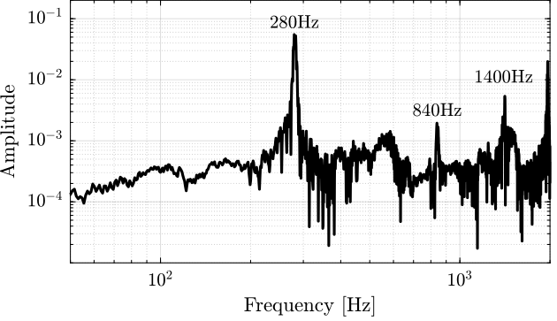
Figure 22: Obtained FRF for the X-bending
Then the APA is in the “free-free” condition, this bending mode is foreseen to be at 200Hz (Figure 19). We are here in the “fixed-free” condition. If we consider that we therefore double the stiffness associated with this mode, we should obtain a resonance a factor \(\sqrt{2}\) higher than 200Hz which is indeed 280Hz. Not sure this reasoning is correct though.
2.4.4 Y-Bending Mode
The setup to measure the Y-bending is shown in Figure 23.
The impact point of the instrumented hammer is located on the back surface of the top interface (on the back of the 2 measurements points).
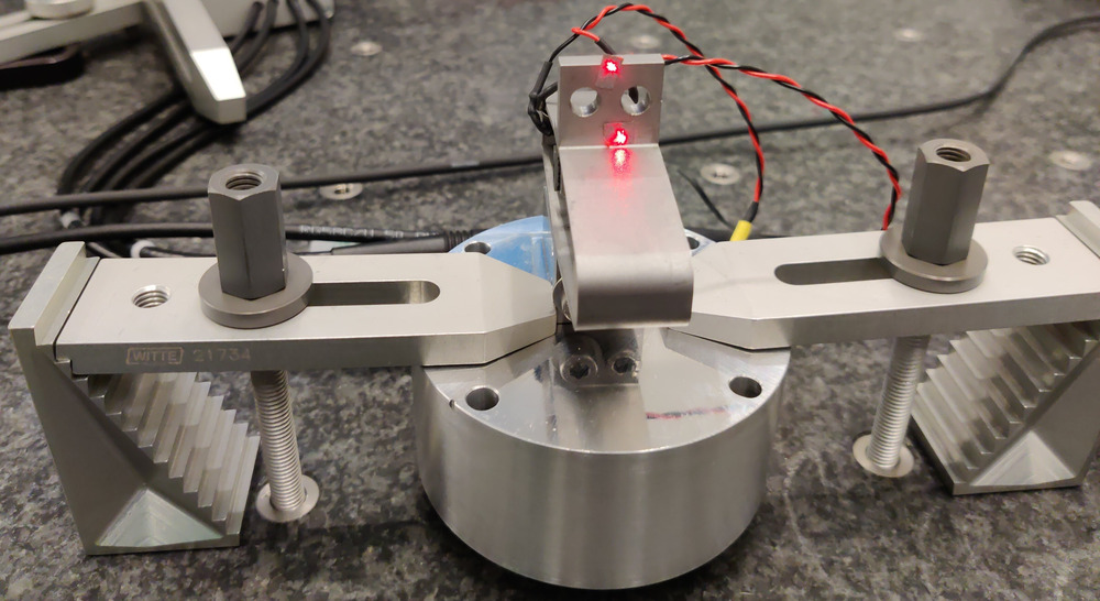
Figure 23: Y-Bending measurement setup
The data is loaded, and the transfer function from the force to the measured rotation is computed.
%% Load Data
bending_Y = load('apa300ml_bending_Y_top.mat');

%% Compute the transfer function
[G_bending_Y, ~]  = tfestimate(bending_Y.Track1, bending_Y.Track2, win, [], [], 1/Ts);
The results are shown in Figure 24. The main resonance is at 412Hz, and we also see the third “harmonic” at 1220Hz.
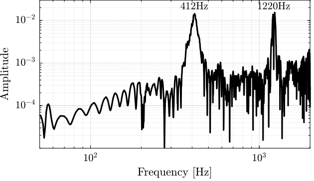
Figure 24: Obtained FRF for the Y-bending
We can apply the same reasoning as in the previous section and estimate the mode to be a factor \(\sqrt{2}\) higher than the mode estimated in the “free-free” condition. We would obtain a mode at 403Hz which is very close to the one estimated here.
2.4.5 Z-Torsion Mode
Finally, we measure the Z-torsion resonance as shown in Figure 25.
The excitation is shown on the other side of the APA, on the side to excite the torsion motion.
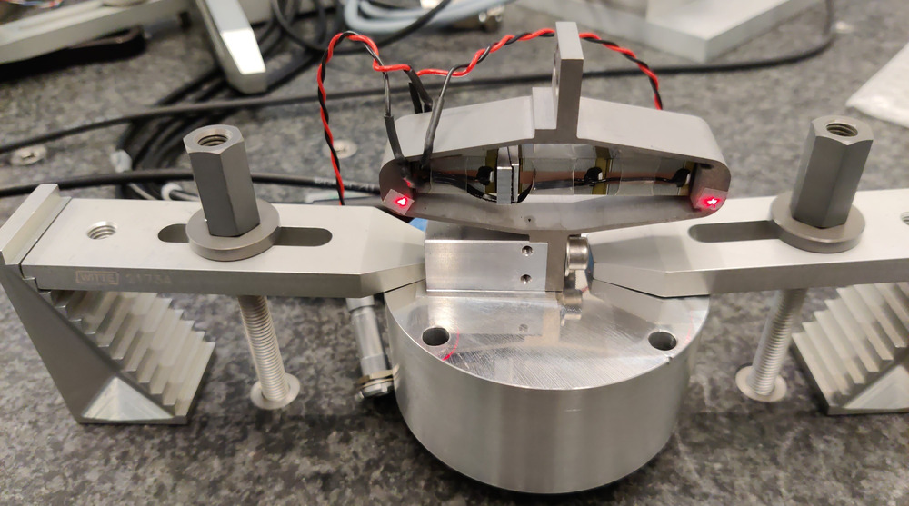
Figure 25: Z-Torsion measurement setup
The data is loaded, and the transfer function computed.
%% Load Data
torsion = load('apa300ml_torsion_left.mat');

%% Compute transfer function
[G_torsion, ~]  = tfestimate(torsion.Track1, torsion.Track2, win, [], [], 1/Ts);
The results are shown in Figure 26. We observe a first peak at 267Hz, which corresponds to the X-bending mode that was measured at 280Hz. And then a second peak at 415Hz, which corresponds to the X-bending mode that was measured at 412Hz. A third mode at 800Hz could correspond to this torsion mode.
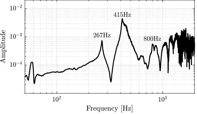
Figure 26: Obtained FRF for the Z-torsion
In order to verify that, the APA is excited on the top part such that the torsion mode should not be excited.
%% Load data
torsion = load('apa300ml_torsion_top.mat');

%% Compute transfer function
[G_torsion_top, ~]  = tfestimate(torsion.Track1, torsion.Track2, win, [], [], 1/Ts);
The two FRF are compared in Figure 27. It is clear that the first two modes does not correspond to the torsional mode. Maybe the resonance at 800Hz, or even higher resonances. It is difficult to conclude here.
Figure 27: Obtained FRF for the Z-torsion
2.4.6 Compare
The three measurements are shown in Figure 28.
Figure 28: Obtained FRF - Comparison
2.4.7 Conclusion
When two flexible joints are fixed at each ends of the APA, the APA is mostly in a free/free condition in terms of bending/torsion (the bending/torsional stiffness of the joints being very small).
In the current tests, the APA are in a fixed/free condition. Therefore, it is quite obvious that we measured higher resonance frequencies than what is foreseen for the struts. It is however quite interesting that there is a factor \(\approx \sqrt{2}\) between the two (increased of the stiffness by a factor 2?).
| Mode | FEM - Strut mode | Measured Frequency |
|---|---|---|
| X-Bending | 189Hz | 280Hz |
| Y-Bending | 285Hz | 410Hz |
| Z-Torsion | 400Hz | 800Hz? |
3 Dynamical measurements - APA
In this section, a measurement test bench is used to extract all the important parameters of the Amplified Piezoelectric Actuator APA300ML.
This include:
- Stroke
- Stiffness
- Hysteresis
- “Actuator constant”: Gain from the applied voltage \(V_a\) to the generated Force \(F_a\)
- “Sensor constant”: Gain from the sensor stack strain \(\delta L\) to the generated voltage \(V_s\)
- Dynamical behavior from the actuator to the force sensor and to the motion of the APA
The bench is shown in Figure 29, and a zoom picture on the APA and encoder is shown in Figure 30.
Figure 29: Picture of the test bench
Figure 30: Zoom on the APA with the encoder
Here are the documentation of the equipment used for this test bench:
- Voltage Amplifier: PD200
- Amplified Piezoelectric Actuator: APA300ML
- DAC/ADC: Speedgoat IO313
- Encoder: Renishaw Vionic and used Ruler
- Interferometer: Attocube IDS3010
The bench is schematically shown in Figure 31 and the signal used are summarized in Table 6.
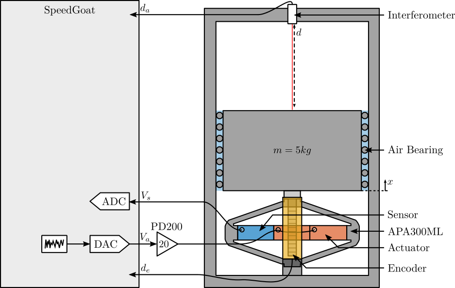
Figure 31: Schematic of the Test Bench
| Variable | Description | Unit | Hardware |
|---|---|---|---|
Va |
Output DAC voltage | [V] | DAC - Ch. 1 - PD200 - APA |
Vs |
Measured stack voltage (ADC) | [V] | APA - ADC - Ch. 1 |
de |
Encoder Measurement | [m] | PEPU Ch. 1 - IO318(1) Ch. 1 |
da |
Attocube Measurement | [m] | PEPU Ch. 2 - IO318(1) Ch. 2 |
t |
Time | [s] |
This section is structured as follows:
3.1 Measurements on APA 1
Measurements are first performed on only one APA. Once the measurement procedure is validated, it is performed on all the other APA.
3.1.1 Excitation Signals
Different excitation signals are used to perform FRF estimations.
Typically, this is done in three steps:
- A low pass filtered white noise is used with rather small amplitudes (Figure 32). This first excitation is used to estimate the main resonance of the system.
- A sweep-sine from 10Hz to 400Hz is used (Figure 33). The sweep-sine is is notched around the estimated resonance of the system.
- A band-limited white noise from 300Hz to 2kHz is used to estimate the high frequency behavior (Figure 34).
For all the excitation signals, before the excitation starts, the mean voltage is slowly increased halfway between the minimum voltage (-20V) and the maximum (150V).
The first measurement is only used to have a first estimation of the dynamics and verify that everything is setup correctly. The second excitation is done to estimate the dynamics from 10Hz to 350Hz and the third excitation from 350Hz to 2kHz. The second and third measurements are therefore combined in the frequency domain to form one good estimation of the dynamics from 10Hz up to 2kHz.
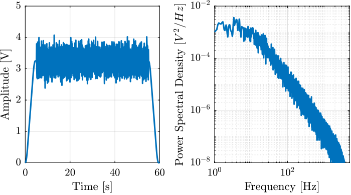
Figure 32: Low pass filtered white noise. Time domain (left), Frequency domain (right)
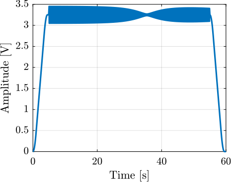
Figure 33: Sweep Sine with a decreased amplitude around the resonance of the APA
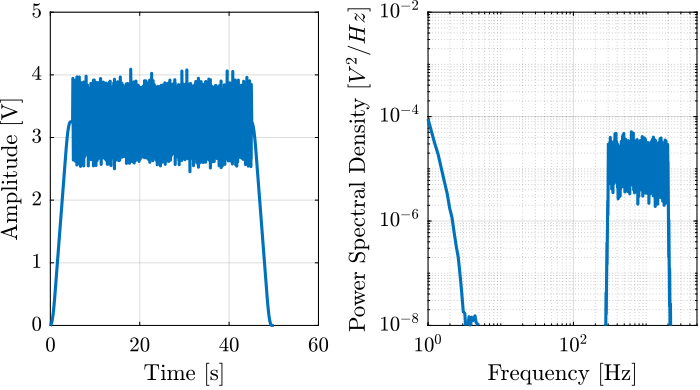
Figure 34: Band-pass white noise. Time domain (left), Frequency domain (right)
3.1.2 First Measurement
For this first measurement for the first APA, a basic logarithmic sweep is used between 10Hz and 2kHz.
The data are loaded.
%% Load data
apa_sweep = load(sprintf('mat/frf_data_%i_sweep.mat', 1), 't', 'Va', 'Vs', 'da', 'de');
The initial time is set to zero.
%% Time vector
t = apa_sweep.t - apa_sweep.t(1) ; % Time vector [s]
The excitation signal is shown in Figure 35. It is a sweep sine from 10Hz up to 2kHz filtered with a notch centered with the main resonance of the system and a low pass filter.
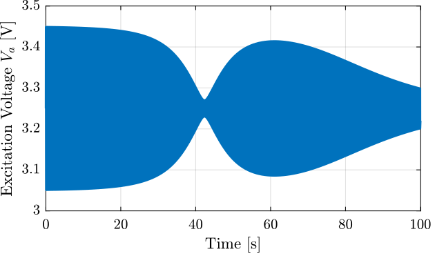
Figure 35: Excitation voltage
3.1.3 FRF - Setup
Let’s define the sampling time/frequency.
%% Sampling Frequency / Time
Ts = (t(end) - t(1))/(length(t)-1); % Sampling Time [s]
Fs = 1/Ts; % Sampling Frequency [Hz]
Then we defined a “Hanning” windows that will be used for the spectral analysis:
win = hanning(ceil(1*Fs)); % Hannning Windows
We get the frequency vector that will be the same for all the frequency domain analysis.
% Only used to have the frequency vector "f"
[~, f] = tfestimate(apa_sweep.Va, apa_sweep.de, win, [], [], 1/Ts);
3.1.4 FRF - Encoder and Interferometer
In this section, the transfer function from the excitation voltage \(V_a\) to the encoder measured displacement \(d_e\) and interferometer measurement \(d_a\).
The coherence from \(V_a\) to \(d_e\) and from \(V_a\) to \(d_a\) are computed and shown in Figure 36. They are quite good from 10Hz up to 500Hz.
%% Compute the coherence
[enc_coh, ~] = mscohere(apa_sweep.Va, apa_sweep.de, win, [], [], 1/Ts);
[int_coh, ~] = mscohere(apa_sweep.Va, apa_sweep.da, win, [], [], 1/Ts);
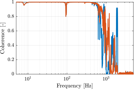
Figure 36: Coherence for the identification from \(V_a\) to \(d_e\)
The transfer functions are then estimated and shown in Figure 37.
%% TF - Encoder and interferometer
[frf_enc, ~] = tfestimate(apa_sweep.Va, apa_sweep.de, win, [], [], 1/Ts);
[frf_int, ~] = tfestimate(apa_sweep.Va, apa_sweep.da, win, [], [], 1/Ts);
It is shown than both the encoder and interferometers are measuring the same dynamics up to \(\approx 700\,Hz\). Above that, it is possible that there is some flexible elements apart from the APA that is adding resonances into one or the other FRF.
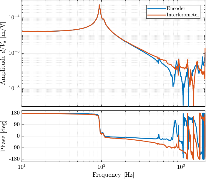
Figure 37: Obtained transfer functions from \(V_a\) to both \(d_e\) and \(d_a\)
The transfer functions obtained in Figure 37 are very close to what was expected:
- constant gain at low frequency
- resonance at around 100Hz which corresponds to the APA axial mode
- no further resonance up until high frequency (\(\approx 700\,Hz\)) at which points several elements of the test bench can induces resonances in the measured FRF
However, it was not expected to observe a “double resonance” at around 95Hz (instead of only one resonance).
3.1.5 FRF - Force Sensor
Now the dynamics from excitation voltage \(V_a\) to the force sensor stack voltage \(V_s\) is identified.
The coherence is computed and shown in Figure 38 and found very good from 10Hz up to 2kHz.
%% Compute the coherence from Va to Vs
[iff_coh, ~] = mscohere(apa_sweep.Va, apa_sweep.Vs, win, [], [], 1/Ts);
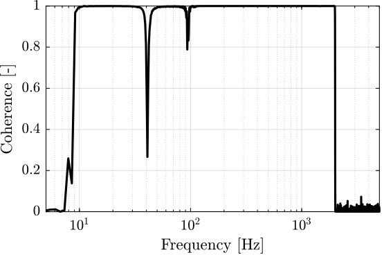
Figure 38: Coherence for the identification from \(V_a\) to \(V_s\)
The transfer function is estimated and shown in Figure 39.
%% Compute the TF from Va to Vs
[iff_sweep, ~] = tfestimate(apa_sweep.Va, apa_sweep.Vs, win, [], [], 1/Ts);
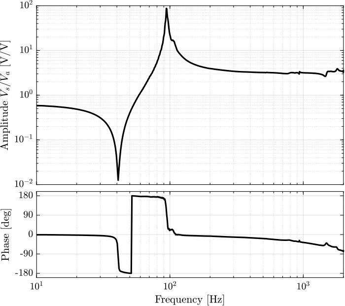
Figure 39: Obtained transfer functions from \(V_a\) to \(V_s\)
The obtained dynamics from the excitation voltage \(V_a\) to the measured sensor stack voltage \(V_s\) is corresponding to what was expected:
- constant gain at low frequency
- complex conjugate zero and then complex conjugate pole
- constant gain at high frequency
3.1.6 Hysteresis
We here wish to visually see the amount of hysteresis present in the APA.
To do so, a quasi static sinusoidal excitation \(V_a\) at different voltages is used.
The offset is 65V (halfway between -20V and 150V), and the sin amplitude is ranging from 1V up to 80V (full range).
For each excitation amplitude, the vertical displacement \(d\) of the mass is measured.
Then, \(d\) is plotted as a function of \(V_a\) for all the amplitudes.
We expect to obtained something like the hysteresis shown in Figure 40.
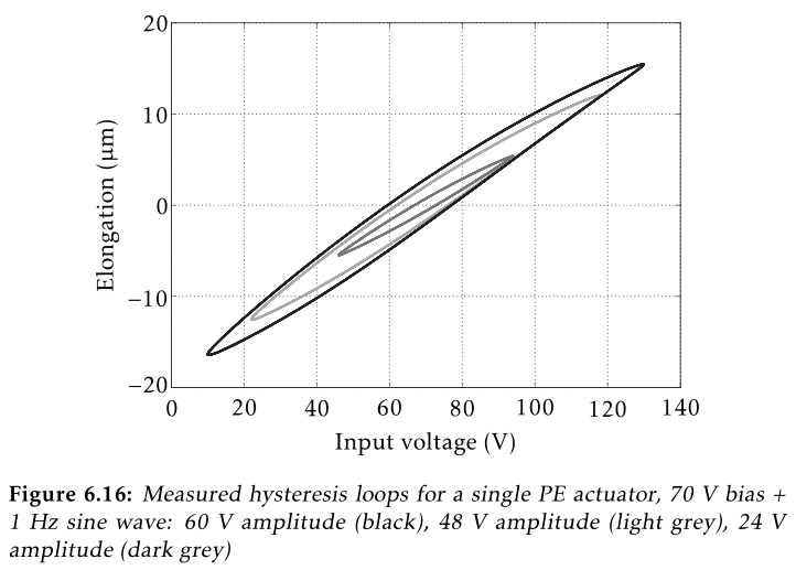
Figure 40: Expected Hysteresis poel10_explor_activ_hard_mount_vibrat
The data is loaded.
%% Load measured data - hysteresis
apa_hyst = load('frf_data_1_hysteresis.mat', 't', 'Va', 'de');
% Initial time set to zero
apa_hyst.t = apa_hyst.t - apa_hyst.t(1);
The excitation voltage amplitudes are:
ampls = [0.1, 0.2, 0.4, 1, 2, 4]; % Excitation voltage amplitudes
The excitation voltage and the measured displacement are shown in Figure 41.
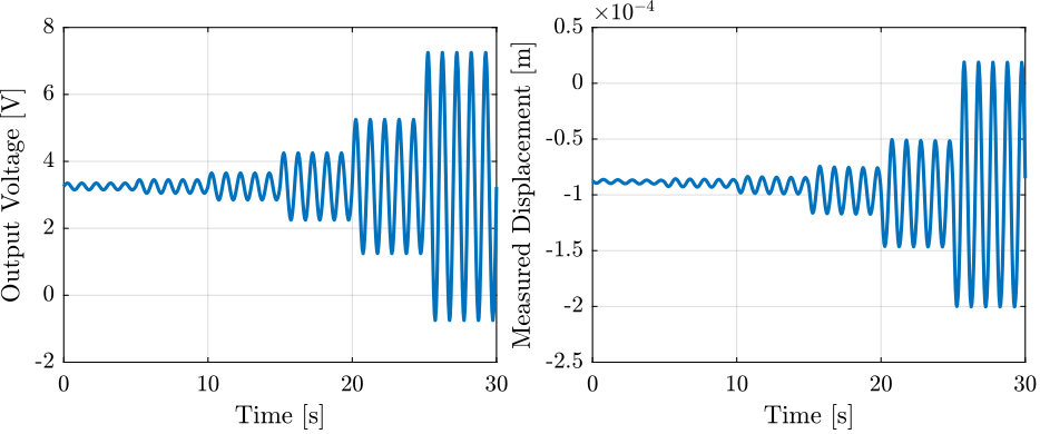
Figure 41: Excitation voltage and measured displacement
For each amplitude, we only take the last sinus in order to reduce possible transients. Also, the motion is centered on zero.
The measured displacement at a function of the output voltage are shown in Figure 42.
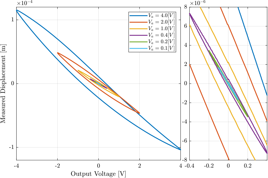
Figure 42: Obtained hysteresis for multiple excitation amplitudes
From Figure 42, it is quite clear that hysteresis is increasing with the excitation amplitude. For small excitation amplitudes (\(V_a < 0.4\,V\)) the hysteresis stays reasonably small.
Also, it is quite interesting to see that no hysteresis is found on the sensor stack voltage when using the same excitation signal.
3.1.7 Estimation of the APA axial stiffness
In order to estimate the stiffness of the APA, a weight with known mass \(m_a\) is added on top of the suspended granite and the deflection \(d_e\) is measured using the encoder.
The APA stiffness can then be estimated to be:
\begin{equation} k_{\text{apa}} = \frac{m_a g}{d} \end{equation}The data is loaded, and the measured displacement is shown in Figure 43.
%% Load data for stiffness measurement
apa_mass = load(sprintf('frf_data_%i_add_mass_closed_circuit.mat', 1), 't', 'de');
apa_mass.de = apa_mass.de - mean(apa_mass.de(apa_mass.t<11));
Figure 43: Measured displacement when adding the mass and removing the mass
From Figure 43, it can be seen that there are some drifts that are probably due to some creep. This will induce some uncertainties in the measured stiffness.
Here, a mass of 6.4 kg was used:
added_mass = 6.4; % Added mass [kg]
The stiffness is then computed as follows:
k = 9.8 * added_mass / (mean(apa_mass.de(apa_mass.t > 12 & apa_mass.t < 12.5)) - mean(apa_mass.de(apa_mass.t > 20 & apa_mass.t < 20.5)));
And the stiffness obtained is very close to the one specified in the documentation (\(k = 1.794\,[N/\mu m]\)).
k = 1.68 [N/um]
The stiffness could also be estimated based on the main vertical resonance of the system at \(\omega_z = 2\pi \cdot 94 \,[rad/s]\). The suspended mass is \(m_{\text{sus}} = 5\,kg\). And therefore, the axial stiffness of the APA can be estimated to be:
\begin{equation} k_{\text{APA}} = m_{\text{sus}} \omega_z^2 \end{equation}wz = 2*pi*94; % [rad/s] msus = 5.7; % [kg] k = msus * wz^2;
k = 1.99 [N/um]
The two values are found relatively close to each other. Anyway, the stiffness of the model will be tuned to match the measured FRF.
3.1.8 Stiffness change due to electrical connections
Changes in the electrical impedance connected to the piezoelectric actuator causes changes in the mechanical compliance (or stiffness) of the piezoelectric actuator.
In this section is measured the stiffness of the APA whether the piezoelectric actuator is connected to an open circuit or a short circuit (e.g. the output of a voltage amplifier).
Note here that the resistor in parallel to the sensor stack is present in both cases.
First, the data are loaded.
%% Load Data
add_mass_oc = load(sprintf('frf_data_%i_add_mass_open_circuit.mat',   1), 't', 'de');
add_mass_cc = load(sprintf('frf_data_%i_add_mass_closed_circuit.mat', 1), 't', 'de');
And the initial displacement is set to zero.
%% Zero displacement at initial time
add_mass_oc.de = add_mass_oc.de - mean(add_mass_oc.de(add_mass_oc.t<11));
add_mass_cc.de = add_mass_cc.de - mean(add_mass_cc.de(add_mass_cc.t<11));
The measured displacements are shown in Figure 44.
Figure 44: Measured displacement
And the stiffness is estimated in both case. The results are shown in Table 7.
apa_k_oc = 9.8 * added_mass / (mean(add_mass_oc.de(add_mass_oc.t > 12 & add_mass_oc.t < 12.5)) - mean(add_mass_oc.de(add_mass_oc.t > 20 & add_mass_oc.t < 20.5)));
apa_k_cc = 9.8 * added_mass / (mean(add_mass_cc.de(add_mass_cc.t > 12 & add_mass_cc.t < 12.5)) - mean(add_mass_cc.de(add_mass_cc.t > 20 & add_mass_cc.t < 20.5)));
| \(k [N/\mu m]\) | |
|---|---|
| Not connected | 2.3 |
| Connected | 1.7 |
Clearly, connecting the actuator stacks to the amplified (basically equivalent as to short circuiting them) lowers its stiffness.
3.1.9 Effect of the resistor on the IFF Plant
A resistor \(R \approx 80.6\,k\Omega\) is added in parallel with the sensor stack. This has the effect to form a high pass filter with the capacitance of the stack.
This is done for two reasons (explained in details this document):
- Limit the voltage offset due to the input bias current of the ADC
- Limit the low frequency gain
The (low frequency) transfer function from \(V_a\) to \(V_s\) with and without this resistor have been measured.
%% Load the data
wi_k = load('frf_data_1_sweep_lf_with_R.mat', 't', 'Vs', 'Va'); % With the resistor
wo_k = load('frf_data_1_sweep_lf.mat',        't', 'Vs', 'Va'); % Without the resistor
We use a very long “Hanning” window for the spectral analysis in order to estimate the low frequency behavior.
win = hanning(ceil(50*Fs)); % Hannning Windows
And we estimate the transfer function from \(V_a\) to \(V_s\) in both cases:
%% Compute the transfer functions from Va to Vs
[frf_wo_k, f] = tfestimate(wo_k.Va, wo_k.Vs, win, [], [], 1/Ts);
[frf_wi_k, ~] = tfestimate(wi_k.Va, wi_k.Vs, win, [], [], 1/Ts);
With the following values of the resistor and capacitance, we obtain a first order high pass filter with a crossover frequency equal to:
%% Model for the high pass filter
C = 5.1e-6; % Sensor Stack capacitance [F]
R = 80.6e3; % Parallel Resistor [Ohm]

f0 = 1/(2*pi*R*C); % Crossover frequency of RC HPF [Hz]
f0 = 0.39 [Hz]
The transfer function of the corresponding high pass filter is:
G_hpf = 0.6*(s/2*pi*f0)/(1 + s/2*pi*f0);
Let’s compare the transfer function from actuator stack to sensor stack with and without the added resistor in Figure 45.
Figure 45: Transfer function from \(V_a\) to \(V_s\) with and without the resistor \(k\)
The added resistor has indeed the expected effect of forming an high pass filter.
3.2 Comparison of all the APA
The same measurements that was performed in Section 3.1 are now performed on all the APA and then compared.
3.2.1 Axial Stiffnesses - Comparison
Let’s first compare the APA axial stiffnesses.
The added mass is:
added_mass = 6.4; % Added mass [kg]
Here are the numbers of the APA that have been measured:
apa_nums = [1 2 4 5 6 7 8];
The data are loaded.
%% Load Data
apa_mass = {};
for i = 1:length(apa_nums)
    apa_mass(i) = {load(sprintf('frf_data_%i_add_mass_closed_circuit.mat', apa_nums(i)), 't', 'de')};
    % The initial displacement is set to zero
    apa_mass{i}.de = apa_mass{i}.de - mean(apa_mass{i}.de(apa_mass{i}.t<11));
end
The raw measurements are shown in Figure 46. All the APA seems to have similar stiffness except the APA 7 which show strange behavior.
It is however strange that the displacement \(d_e\) when the mass is removed is higher for the APA 7 than for the other APA. What could cause that? It is probably due to the fact that the mechanical element holding the granite in place was not removed.
Figure 46: Raw measurements for all the APA. A mass of 6.4kg is added at arround 15s and removed at arround 22s
The stiffnesses are computed for all the APA and are summarized in Table 8.
| APA Num | \(k [N/\mu m]\) |
|---|---|
| 1 | 1.68 |
| 2 | 1.69 |
| 4 | 1.7 |
| 5 | 1.7 |
| 6 | 1.7 |
| 7 | 1.93 |
| 8 | 1.73 |
The APA300ML manual specifies the nominal stiffness to be \(1.8\,[N/\mu m]\) which is very close to what have been measured. Only the APA number 7 is a little bit off, maybe there was a problem with the experimental setup.
3.2.2 FRF - Setup
The identification is performed in three steps:
- White noise excitation with small amplitude. This is used to determine the main resonance of the system.
- Sweep sine excitation with the amplitude lowered around the resonance. The sweep sine is from 10Hz to 400Hz.
- High frequency noise. The noise is band-passed between 300Hz and 2kHz.
Then, the result of the second identification is used between 10Hz and 350Hz and the result of the third identification if used between 350Hz and 2kHz.
The data are loaded for both the second and third identification:
%% Second identification
apa_sweep = {};
for i = 1:length(apa_nums)
    apa_sweep(i) = {load(sprintf('frf_data_%i_sweep.mat', apa_nums(i)), 't', 'Va', 'Vs', 'de', 'da')};
end

%% Third identification
apa_noise_hf = {};
for i = 1:length(apa_nums)
    apa_noise_hf(i) = {load(sprintf('frf_data_%i_noise_hf.mat', apa_nums(i)), 't', 'Va', 'Vs', 'de', 'da')};
end
The time is the same for all measurements.
%% Time vector
t = apa_sweep{1}.t - apa_sweep{1}.t(1) ; % Time vector [s]

%% Sampling
Ts = (t(end) - t(1))/(length(t)-1); % Sampling Time [s]
Fs = 1/Ts; % Sampling Frequency [Hz]
Then we defined a “Hanning” windows that will be used for the spectral analysis:
win = hanning(ceil(0.5*Fs)); % Hannning Windows
We get the frequency vector that will be the same for all the frequency domain analysis.
% Only used to have the frequency vector "f"
[~, f] = tfestimate(apa_sweep{1}.Va, apa_sweep{1}.de, win, [], [], 1/Ts);
i_lf = f <= 350;
i_hf = f >  350;
3.2.3 FRF - Encoder and Interferometer
In this section, the dynamics from excitation voltage \(V_a\) to encoder measured displacement \(d_e\) is identified.
We compute the coherence for 2nd and 3rd identification:
%% Coherence computation
coh_enc = zeros(length(f), length(apa_nums));
for i = 1:length(apa_nums)
    [coh_lf, ~] = mscohere(apa_sweep{i}.Va,    apa_sweep{i}.de,    win, [], [], 1/Ts);
    [coh_hf, ~] = mscohere(apa_noise_hf{i}.Va, apa_noise_hf{i}.de, win, [], [], 1/Ts);
    coh_enc(:, i) = [coh_lf(i_lf); coh_hf(i_hf)];
end
The coherence is shown in Figure 47, and it is found that the coherence is good from low frequency up to 700Hz.
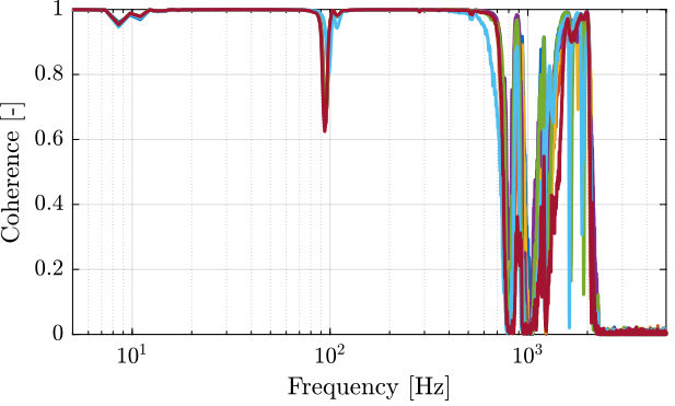
Figure 47: Obtained coherence for the plant from \(V_a\) to \(d_e\)
Then, the transfer function from the DAC output voltage \(V_a\) to the measured displacement by the encoders is computed:
%% Transfer function estimation
enc_frf = zeros(length(f), length(apa_nums));
for i = 1:length(apa_nums)
    [frf_lf, ~] = tfestimate(apa_sweep{i}.Va,    apa_sweep{i}.de,    win, [], [], 1/Ts);
    [frf_hf, ~] = tfestimate(apa_noise_hf{i}.Va, apa_noise_hf{i}.de, win, [], [], 1/Ts);
    enc_frf(:, i) = [frf_lf(i_lf); frf_hf(i_hf)];
end
The obtained transfer functions are shown in Figure 48. They are all superimposed except for the APA7.
Why is the APA7 dynamical behavior is so different from the other? We could think that the APA7 is stiffer, but also the mass line is off, and it should indeed be identical.
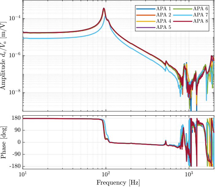
Figure 48: Estimated FRF for the DVF plant (transfer function from \(V_a\) to the encoder \(d_e\))
A zoom on the main resonance is shown in Figure 49. It is clear that expect for the APA 7, the response around the resonances are well matching for all the APA.
It is also clear that there is not a single resonance but two resonances, a first one at 95Hz and a second one at 105Hz.
Why is there a double resonance at around 94Hz?
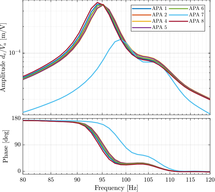
Figure 49: Estimated FRF for the DVF plant (transfer function from \(V_a\) to the encoder \(d_e\)) - Zoom on the main resonance
3.2.4 FRF - Force Sensor
In this section, the dynamics from \(V_a\) to \(V_s\) is identified.
First the coherence is computed and shown in Figure 50. The coherence is very nice from 10Hz to 2kHz. It is only dropping near a zeros at 40Hz, and near the resonance at 95Hz (the excitation amplitude being lowered).
%% Compute the Coherence
coh_iff = zeros(length(f), length(apa_nums));
for i = 1:length(apa_nums)
    [coh_lf, ~] = mscohere(apa_sweep{i}.Va,    apa_sweep{i}.Vs,    win, [], [], 1/Ts);
    [coh_hf, ~] = mscohere(apa_noise_hf{i}.Va, apa_noise_hf{i}.Vs, win, [], [], 1/Ts);
    coh_iff(:, i) = [coh_lf(i_lf); coh_hf(i_hf)];
end
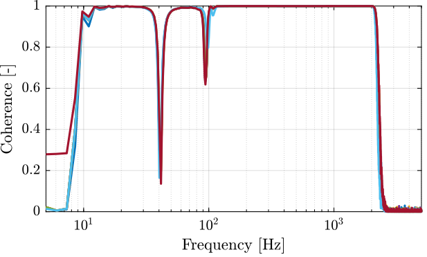
Figure 50: Obtained coherence for the IFF plant
Then the FRF are estimated and shown in Figure 51
%% FRF estimation of the transfer function from Va to Vs
iff_frf = zeros(length(f), length(apa_nums));
for i = 1:length(apa_nums)
    [frf_lf, ~] = tfestimate(apa_sweep{i}.Va,    apa_sweep{i}.Vs,    win, [], [], 1/Ts);
    [frf_hf, ~] = tfestimate(apa_noise_hf{i}.Va, apa_noise_hf{i}.Vs, win, [], [], 1/Ts);
    iff_frf(:, i) = [frf_lf(i_lf); frf_hf(i_hf)];
end
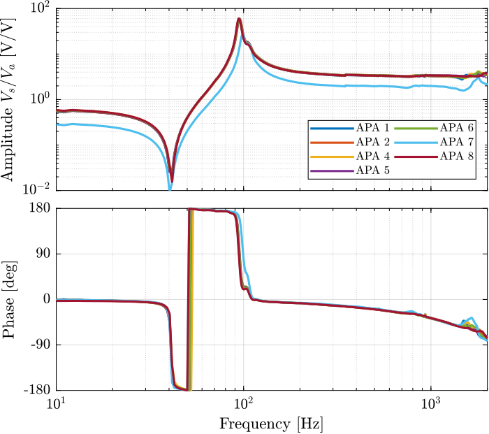
Figure 51: Identified IFF Plant
3.2.5 Conclusion
Except the APA 7 which shows strange behavior, all the other APA are showing a very similar behavior.
So far, all the measured FRF are showing the dynamical behavior that was expected.
%% Remove the APA 7 (6 in the list) from measurements
apa_nums(6) = [];
enc_frf(:,6) = [];
iff_frf(:,6) = [];
%% Save the measured FRF
save('mat/meas_apa_frf.mat', 'f', 'Ts', 'enc_frf', 'iff_frf', 'apa_nums');
4 Test Bench APA300ML - Simscape Model
In this section, a simscape model (Figure 52) of the measurement bench is used to compare the model of the APA with the measured FRF.
After the transfer functions are extracted from the model (Section 4.1), the comparison of the obtained dynamics with the measured FRF will permit to:
- Estimate the “actuator constant” and “sensor constant” (Section 4.2)
- Tune the model of the APA to match the measured dynamics (Section 4.3)
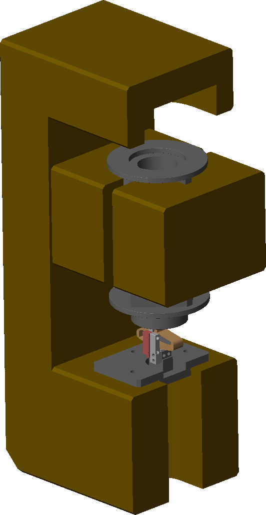
Figure 52: Screenshot of the Simscape model
4.1 First Identification
The APA is first initialized with default parameters:
%% Initialize the structure with default values
n_hexapod = struct();
n_hexapod.actuator = initializeAPA(...
    'type', '2dof', ...
    'Ga', 1, ... % Actuator constant [N/V]
    'Gs', 1);    % Sensor constant [V/m]
The transfer function from excitation voltage \(V_a\) (before the amplification of \(20\) due to the PD200 amplifier) to:
- the sensor stack voltage \(V_s\)
- the measured displacement by the encoder \(d_e\)
- the measured displacement by the interferometer \(d_a\)
%% Input/Output definition
clear io; io_i = 1;
io(io_i) = linio([mdl, '/Va'],  1, 'openinput');  io_i = io_i + 1; % DAC Voltage
io(io_i) = linio([mdl, '/Vs'],  1, 'openoutput'); io_i = io_i + 1; % Sensor Voltage
io(io_i) = linio([mdl, '/de'],  1, 'openoutput'); io_i = io_i + 1; % Encoder
io(io_i) = linio([mdl, '/da'],  1, 'openoutput'); io_i = io_i + 1; % Interferometer

%% Run the linearization
Ga = linearize(mdl, io, 0.0, options);
Ga.InputName  = {'Va'};
Ga.OutputName = {'Vs', 'de', 'da'};
The obtain dynamics are shown in Figure 53 and 54. It can be seen that:
- the shape of these bode plots are very similar to the one measured in Section 3 expect from a change in gain and exact location of poles and zeros
- there is a sign error for the transfer function from \(V_a\) to \(V_s\). This will be corrected by taking a negative “sensor gain”.
- the low frequency zero of the transfer function from \(V_a\) to \(V_s\) is minimum phase as expected. The measured FRF are showing non-minimum phase zero, but it is most likely due to measurements artifacts.

Figure 53: Bode plot of the transfer function from \(V_a\) to \(V_s\)
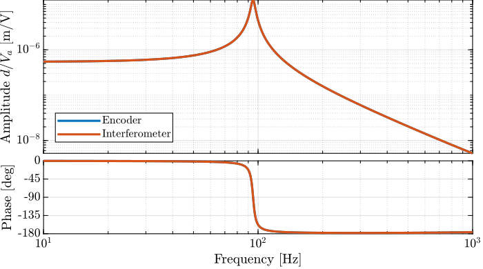
Figure 54: Bode plot of the transfer function from \(V_a\) to \(d_L\) and to \(z\)
4.2 Identify Sensor/Actuator constants and compare with measured FRF
4.2.1 How to identify these constants?
4.2.1.1 Piezoelectric Actuator Constant
Using the measurement test-bench, it is rather easy the determine the static gain between the applied voltage \(V_a\) to the induced displacement \(d\).
\begin{equation} d = g_{d/V_a} \cdot V_a \end{equation}Using the Simscape model of the APA, it is possible to determine the static gain between the actuator force \(F_a\) to the induced displacement \(d\):
\begin{equation} d = g_{d/F_a} \cdot F_a \end{equation}From the two gains, it is then easy to determine \(g_a\):
\begin{equation} \label{eq:actuator_constant_formula} \boxed{g_a = \frac{F_a}{V_a} = \frac{F_a}{d} \cdot \frac{d}{V_a} = \frac{g_{d/V_a}}{g_{d/F_a}}} \end{equation}4.2.1.2 Piezoelectric Sensor Constant
Similarly, it is easy to determine the gain from the excitation voltage \(V_a\) to the voltage generated by the sensor stack \(V_s\):
\begin{equation} V_s = g_{V_s/V_a} V_a \end{equation}Note here that there is an high pass filter formed by the piezoelectric capacitor and parallel resistor.
The gain can be computed from the dynamical identification and taking the gain at the wanted frequency (above the first resonance).
Using the simscape model, compute the gain at the same frequency from the actuator force \(F_a\) to the strain of the sensor stack \(dl\):
\begin{equation} dl = g_{dl/F_a} F_a \end{equation}Then, the “sensor” constant is:
\begin{equation} \label{eq:sensor_constant_formula} \boxed{g_s = \frac{V_s}{dl} = \frac{V_s}{V_a} \cdot \frac{V_a}{F_a} \cdot \frac{F_a}{dl} = \frac{g_{V_s/V_a}}{g_a \cdot g_{dl/F_a}}} \end{equation}4.2.2 Identification Data
Let’s load the measured FRF from the DAC voltage to the measured encoder and to the sensor stack voltage.
%% Load Data
load('meas_apa_frf.mat', 'f', 'Ts', 'enc_frf', 'iff_frf', 'apa_nums');
4.2.3 2DoF APA
4.2.3.1 2DoF APA
Let’s initialize the APA as a 2DoF model with unity sensor and actuator gains.
%% Initialize a 2DoF APA with Ga=Gs=1
n_hexapod.actuator = initializeAPA(...
    'type', '2dof', ...
    'ga', 1, ...
    'gs', 1);
4.2.3.2 Identification without actuator or sensor constants
The transfer function from \(V_a\) to \(V_s\), \(d_e\) and \(d_a\) is identified.
%% Input/Output definition
clear io; io_i = 1;
io(io_i) = linio([mdl, '/Va'], 1, 'openinput');  io_i = io_i + 1; % Actuator Voltage
io(io_i) = linio([mdl, '/Vs'], 1, 'openoutput'); io_i = io_i + 1; % Sensor Voltage
io(io_i) = linio([mdl, '/de'], 1, 'openoutput'); io_i = io_i + 1; % Encoder
io(io_i) = linio([mdl, '/da'], 1, 'openoutput'); io_i = io_i + 1; % Attocube

%% Identification
Gs = linearize(mdl, io, 0.0, options);
Gs.InputName  = {'Va'};
Gs.OutputName = {'Vs', 'de', 'da'};
4.2.3.3 Actuator Constant
Then, the actuator constant can be computed as shown in Eq. \eqref{eq:actuator_constant_formula} by dividing the measured DC gain of the transfer function from \(V_a\) to \(d_e\) by the estimated DC gain of the transfer function from \(V_a\) (in truth the actuator force called \(F_a\)) to \(d_e\) using the Simscape model.
%% Estimated Actuator Constant
ga = -mean(abs(enc_frf(f>10 & f<20)))./dcgain(Gs('de', 'Va')); % [N/V]
ga = -32.2 [N/V]
4.2.3.4 Sensor Constant
Similarly, the sensor constant can be estimated using Eq. \eqref{eq:sensor_constant_formula}.
%% Estimated Sensor Constant
gs = -mean(abs(iff_frf(f>400 & f<500)))./(ga*abs(squeeze(freqresp(Gs('Vs', 'Va'), 1e3, 'Hz')))); % [V/m]
gs = 0.088 [V/m]
4.2.3.5 Comparison
Let’s now initialize the APA with identified sensor and actuator constant:
%% Set the identified constants
n_hexapod.actuator = initializeAPA(...
    'type', '2dof', ...
    'ga', ga, ... % Actuator gain [N/V]
    'gs', gs);    % Sensor gain [V/m]
And identify the dynamics with included constants.
%% Identify again the dynamics with correct Ga,Gs
Gs = linearize(mdl, io, 0.0, options);
Gs = Gs*exp(-Ts*s);
Gs.InputName  = {'Va'};
Gs.OutputName = {'Vs', 'de', 'da'};
The transfer functions from \(V_a\) to \(d_e\) are compared in Figure 55 and the one from \(V_a\) to \(V_s\) are compared in Figure 56.
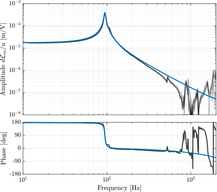
Figure 55: Comparison of the experimental data and Simscape model (\(V_a\) to \(d_e\))
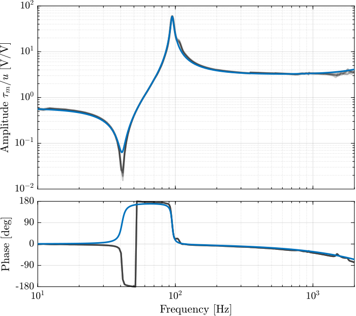
Figure 56: Comparison of the experimental data and Simscape model (\(V_a\) to \(V_s\))
The “actuator constant” and “sensor constant” can indeed be identified using this test bench. After identifying these constants, the 2DoF model shows good agreement with the measured dynamics.
4.2.4 Flexible APA
In this section, the sensor and actuator “constants” are also estimated for the flexible model of the APA.
4.2.4.1 Flexible APA
The Simscape APA model is initialized as a flexible one with unity “constants”.
%% Initialize the APA as a flexible body
n_hexapod.actuator = initializeAPA(...
    'type', 'flexible', ...
    'ga', 1, ...
    'gs', 1);
4.2.4.2 Identification without actuator or sensor constants
The dynamics from \(V_a\) to \(V_s\), \(d_e\) and \(d_a\) is identified.
%% Identify the dynamics
Gs = linearize(mdl, io, 0.0, options);
Gs.InputName  = {'Va'};
Gs.OutputName = {'Vs', 'de', 'da'};
4.2.4.3 Actuator Constant
Then, the actuator constant can be computed as shown in Eq. \eqref{eq:actuator_constant_formula}:
%% Actuator Constant
ga = -mean(abs(enc_frf(f>10 & f<20)))./dcgain(Gs('de', 'Va')); % [N/V]
ga = 23.5 [N/V]
4.2.4.4 Sensor Constant
%% Sensor Constant
gs = -mean(abs(iff_frf(f>400 & f<500)))./(ga*abs(squeeze(freqresp(Gs('Vs', 'Va'), 1e3, 'Hz')))); % [V/m]
gs = -4839841.756 [V/m]
4.2.4.5 Comparison
Let’s now initialize the flexible APA with identified sensor and actuator constant:
%% Set the identified constants
n_hexapod.actuator = initializeAPA(...
    'type', 'flexible', ...
    'ga', ga, ... % Actuator gain [N/V]
    'gs', gs);    % Sensor gain [V/m]
And identify the dynamics with included constants.
%% Identify with updated constants
Gs = linearize(mdl, io, 0.0, options);
Gs = Gs*exp(-Ts*s);
Gs.InputName  = {'Va'};
Gs.OutputName = {'Vs', 'de', 'da'};
The obtained dynamics is compared with the measured one in Figures 57 and 58.
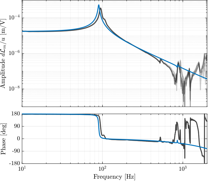
Figure 57: Comparison of the experimental data and Simscape model (\(u\) to \(d\mathcal{L}_m\))
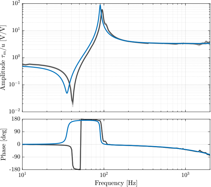
Figure 58: Comparison of the experimental data and Simscape model (\(u\) to \(\tau_m\))
The flexible model is a bit “soft” as compared with the experimental results.
4.3 Optimize 2-DoF model to fit the experimental Data
The parameters of the 2DoF model presented in Section 1.1 are now optimize such that the model best matches the measured FRF.
After optimization, the following parameters are used:
%% Optimized parameters
n_hexapod.actuator = initializeAPA('type', '2dof', ...
                                   'Ga', -32.2, ...
                                   'Gs', 0.088, ...
                                   'k',  ones(6,1)*0.38e6, ...
                                   'ke', ones(6,1)*1.75e6, ...
                                   'ka', ones(6,1)*3e7, ...
                                   'c',  ones(6,1)*1.3e2, ...
                                   'ce', ones(6,1)*1e1, ...
                                   'ca', ones(6,1)*1e1 ...
                                   );
The dynamics is identified using the Simscape model and compared with the measured FRF in Figure 59.
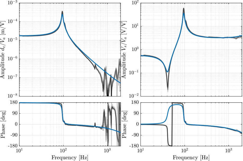
Figure 59: Comparison of the measured FRF and the optimized model
The tuned 2DoF is very well representing the (axial) dynamics of the APA.
5 Dynamical measurements - Struts
The same bench used in Section 3 is here used with the strut instead of only the APA.
The bench is shown in Figure 60. Measurements are performed either when no encoder is fixed to the strut (Figure 61) or when one encoder is fixed to the strut (Figure 62).
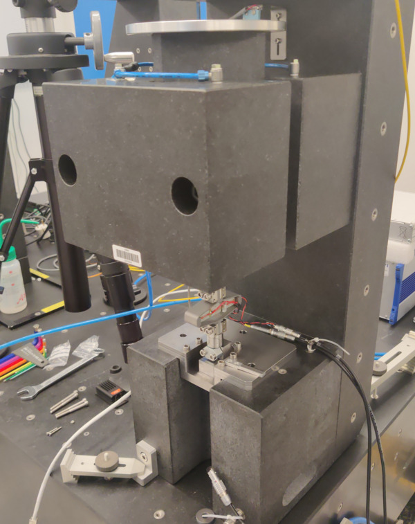
Figure 60: Test Bench with Strut - Overview
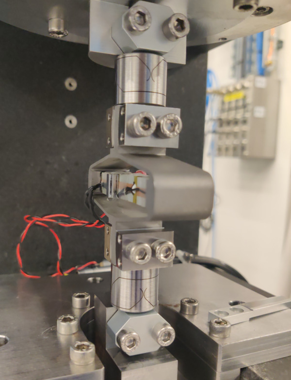
Figure 61: Test Bench with Strut - Zoom on the strut
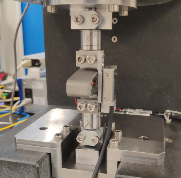
Figure 62: Test Bench with Strut - Zoom on the strut with the encoder
Variables are named the same as in Section 3.
First, only one strut is measured in details (Section 5.1), and then all the struts are measured and compared (Section 5.2).
5.1 Measurement on Strut 1
Measurements are first performed on one of the strut that contains:
- the Amplified Piezoelectric Actuator (APA) number 1
- flexible joints 1 and 2
In Section 5.1.1, the dynamics of the strut is measured without the encoder attached to it. Then in Section 5.1.2, the encoder is attached to the struts, and the dynamic is identified.
5.1.1 Without Encoder
5.1.1.1 FRF Identification - Setup
Similarly to what was done for the identification of the APA, the identification is performed in three steps:
- White noise excitation with small amplitude. This is used to determine the main resonance of the system.
- Sweep sine excitation with the amplitude lowered around the resonance. The sweep sine is from 10Hz to 400Hz.
- High frequency noise. The noise is band-passed between 300Hz and 2kHz.
Then, the result of the second identification is used between 10Hz and 350Hz and the result of the third identification if used between 350Hz and 2kHz.
%% Load Data
leg_sweep    = load(sprintf('frf_data_leg_%i_sweep.mat',    1), 't', 'Va', 'Vs', 'de', 'da');
leg_noise_hf = load(sprintf('frf_data_leg_%i_noise_hf.mat', 1), 't', 'Va', 'Vs', 'de', 'da');
The time is the same for all measurements.
%% Time vector
t = leg_sweep.t - leg_sweep.t(1) ; % Time vector [s]

%% Sampling frequency/time
Ts = (t(end) - t(1))/(length(t)-1); % Sampling Time [s]
Fs = 1/Ts; % Sampling Frequency [Hz]
Then we defined a “Hanning” windows that will be used for the spectral analysis:
win = hanning(ceil(0.5*Fs)); % Hannning Windows
We get the frequency vector that will be the same for all the frequency domain analysis.
% Only used to have the frequency vector "f"
[~, f] = tfestimate(leg_sweep.Va, leg_sweep.de, win, [], [], 1/Ts);
i_lf = f <= 350; % Indices used for the low frequency
i_hf = f >  350; % Indices used for the low frequency
5.1.1.2 FRF Identification - Interferometer
In this section, the dynamics from the excitation voltage \(V_a\) to the interferometer \(d_a\) is identified.
We compute the coherence for 2nd and 3rd identification and combine them.
%% Compute the coherence for both excitation signals
[int_coh_sweep, ~]    = mscohere(leg_sweep.Va,    leg_sweep.da,    win, [], [], 1/Ts);
[int_coh_noise_hf, ~] = mscohere(leg_noise_hf.Va, leg_noise_hf.da, win, [], [], 1/Ts);

%% Combine the coherence
int_coh = [int_coh_sweep(i_lf); int_coh_noise_hf(i_hf)];
The combined coherence is shown in Figure 63, and is found to be very good up to at least 1kHz.
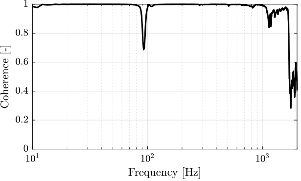
Figure 63: Obtained coherence for the plant from \(V_a\) to \(d_a\)
The transfer function from \(V_a\) to the interferometer measured displacement \(d_a\) is estimated and shown in Figure 64.
%% Compute FRF function from Va to da
[frf_sweep, ~]    = tfestimate(leg_sweep.Va,    leg_sweep.da,    win, [], [], 1/Ts);
[frf_noise_hf, ~] = tfestimate(leg_noise_hf.Va, leg_noise_hf.da, win, [], [], 1/Ts);

%% Combine the FRF
int_frf = [frf_sweep(i_lf); frf_noise_hf(i_hf)];
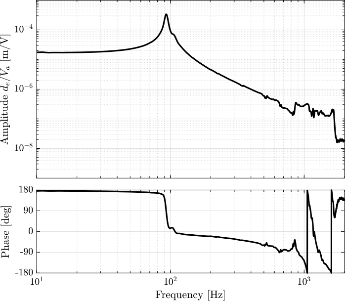
Figure 64: Estimated FRF for the DVF plant (transfer function from \(V_a\) to the interferometer \(d_a\))
5.1.1.3 FRF Identification - IFF
In this section, the dynamics from \(V_a\) to \(V_s\) is identified.
First the coherence is computed and shown in Figure 65. The coherence is very nice from 10Hz to 2kHz. It is only dropping near a zeros at 40Hz, and near the resonance at 95Hz (the excitation amplitude being lowered).
%% Compute the coherence for both excitation signals
[iff_coh_sweep, ~]    = mscohere(leg_sweep.Va,    leg_sweep.Vs,    win, [], [], 1/Ts);
[iff_coh_noise_hf, ~] = mscohere(leg_noise_hf.Va, leg_noise_hf.Vs, win, [], [], 1/Ts);

%% Combine the coherence
iff_coh = [iff_coh_sweep(i_lf); iff_coh_noise_hf(i_hf)];
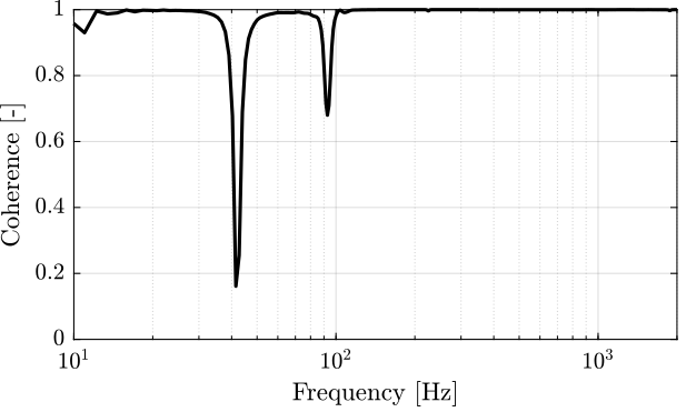
Figure 65: Obtained coherence for the IFF plant
Then the FRF are estimated and shown in Figure 66
%% Compute the FRF
[frf_sweep,    ~] = tfestimate(leg_sweep.Va,    leg_sweep.Vs,    win, [], [], 1/Ts);
[frf_noise_hf, ~] = tfestimate(leg_noise_hf.Va, leg_noise_hf.Vs, win, [], [], 1/Ts);

%% Combine the FRF
iff_frf = [frf_sweep(i_lf); frf_noise_hf(i_hf)];
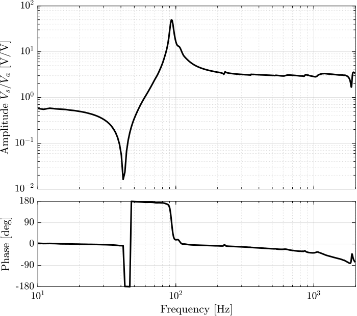
Figure 66: Identified IFF Plant for the Strut 1
5.1.2 With Encoder
5.1.2.1 Measurement Data
The measurements are loaded.
%% Load data
leg_enc_sweep    = load(sprintf('frf_data_leg_coder_badly_align_%i_noise.mat',    1), 't', 'Va', 'Vs', 'de', 'da');
leg_enc_noise_hf = load(sprintf('frf_data_leg_coder_badly_align_%i_noise_hf.mat', 1), 't', 'Va', 'Vs', 'de', 'da');
5.1.2.2 FRF Identification - Interferometer
In this section, the dynamics from \(V_a\) to \(d_a\) is identified.
First, the coherence is computed and shown in Figure 67.
%% Compute the coherence for both excitation signals
[int_coh_sweep, ~]    = mscohere(leg_enc_sweep.Va,    leg_enc_sweep.da,    win, [], [], 1/Ts);
[int_coh_noise_hf, ~] = mscohere(leg_enc_noise_hf.Va, leg_enc_noise_hf.da, win, [], [], 1/Ts);

%% Combine the coherinte
int_coh = [int_coh_sweep(i_lf); int_coh_noise_hf(i_hf)];
Figure 67: Obtained coherence for the plant from \(V_a\) to \(d_a\)
Then the FRF are computed and shown in Figure 68.
%% Compute FRF function from Va to da
[frf_sweep, ~]    = tfestimate(leg_enc_sweep.Va,    leg_enc_sweep.da,    win, [], [], 1/Ts);
[frf_noise_hf, ~] = tfestimate(leg_enc_noise_hf.Va, leg_enc_noise_hf.da, win, [], [], 1/Ts);

%% Combine the FRF
int_with_enc_frf = [frf_sweep(i_lf); frf_noise_hf(i_hf)];
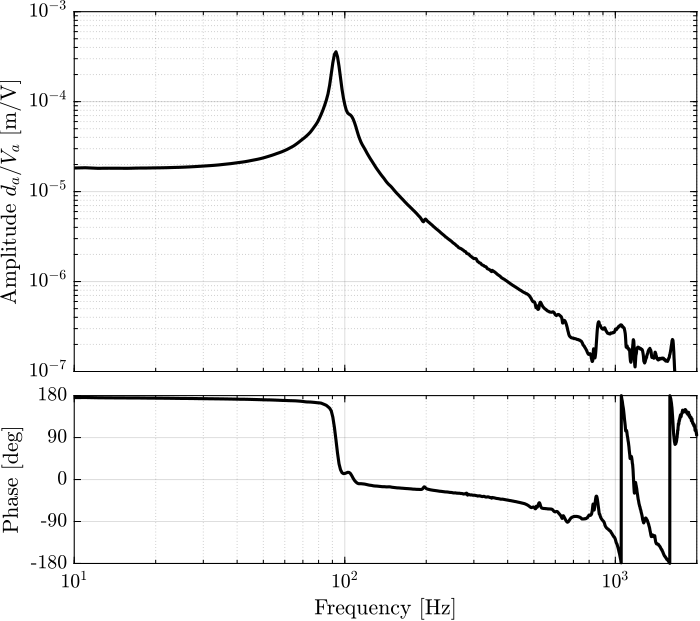
Figure 68: Estimated FRF for the DVF plant (transfer function from \(V_a\) to the encoder \(d_e\))
The obtained FRF is very close to the one that was obtained when no encoder was fixed to the struts as shown in Figure 69.
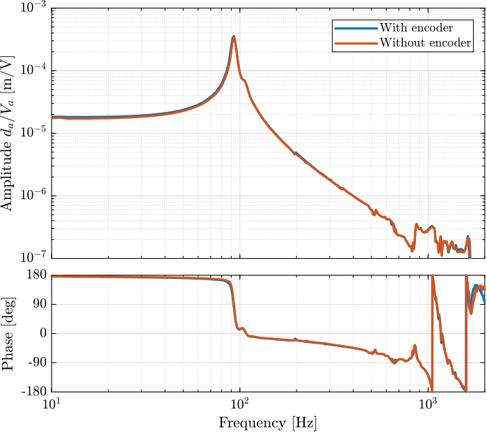
Figure 69: Comparison of the measured FRF from \(V_a\) to \(d_a\) with and without the encoders fixed to the struts
5.1.2.3 FRF Identification - Encoder
In this section, the dynamics from \(V_a\) to \(d_e\) (encoder) is identified.
The coherence is computed and shown in Figure 70.
%% Compute the coherence for both excitation signals
[enc_coh_sweep, ~]    = mscohere(leg_enc_sweep.Va,    leg_enc_sweep.de,    win, [], [], 1/Ts);
[enc_coh_noise_hf, ~] = mscohere(leg_enc_noise_hf.Va, leg_enc_noise_hf.de, win, [], [], 1/Ts);

%% Combine the coherence
enc_coh = [enc_coh_sweep(i_lf); enc_coh_noise_hf(i_hf)];
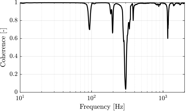
Figure 70: Obtained coherence for the plant from \(V_a\) to \(d_e\) and from \(V_a\) to \(d_a\)
The FRF from \(V_a\) to the encoder measured displacement \(d_e\) is computed and shown in Figure 71.
%% Compute FRF function from Va to da
[frf_sweep, ~]    = tfestimate(leg_enc_sweep.Va,    leg_enc_sweep.de,    win, [], [], 1/Ts);
[frf_noise_hf, ~] = tfestimate(leg_enc_noise_hf.Va, leg_enc_noise_hf.de, win, [], [], 1/Ts);

%% Combine the FRF
enc_frf = [frf_sweep(i_lf); frf_noise_hf(i_hf)];
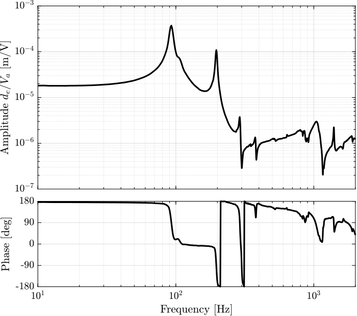
Figure 71: Estimated FRF for the DVF plant (transfer function from \(V_a\) to the encoder \(d_e\))
The transfer functions from \(V_a\) to \(d_e\) (encoder) and to \(d_a\) (interferometer) are compared in Figure 72.
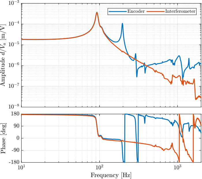
Figure 72: Comparison of the transfer functions from excitation voltage \(V_a\) to either the encoder \(d_e\) or the interferometer \(d_a\)
The dynamics from the excitation voltage \(V_a\) to the measured displacement by the encoder \(d_e\) presents much more complicated behavior than the transfer function to the displacement as measured by the Interferometer (compared in Figure 72). It will be further investigated why the two dynamics as so different and what are causing all these resonances.
5.1.2.4 APA Resonances Frequency
As shown in Figure 73, we can clearly see three spurious resonances at 197Hz, 290Hz and 376Hz.
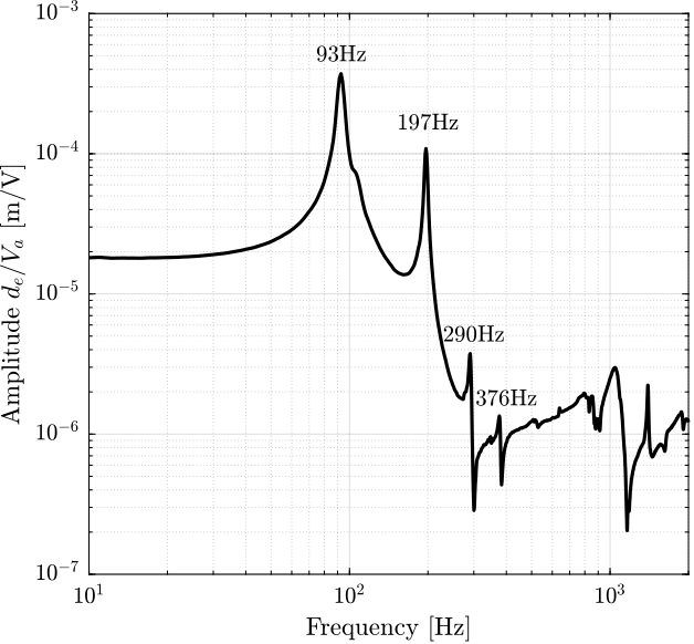
Figure 73: Magnitude of the transfer function from excitation voltage \(V_a\) to encoder measurement \(d_e\). The frequency of the resonances are noted.
These resonances correspond to parasitic resonances of the strut itself.
They are very close to what was estimated using a finite element model of the strut (Figure 74):
- Mode in X-bending at 189Hz
- Mode in Y-bending at 285Hz
- Mode in Z-torsion at 400Hz
Figure 74: Spurious resonances. a) X-bending mode at 189Hz. b) Y-bending mode at 285Hz. c) Z-torsion mode at 400Hz
5.1.2.5 FRF Identification - Force Sensor
In this section, the dynamics from \(V_a\) to \(V_s\) is identified.
First the coherence is computed and shown in Figure 75. The coherence is very nice from 10Hz to 2kHz. It is only dropping near a zeros at 40Hz, and near the resonance at 95Hz (the excitation amplitude being lowered).
%% Compute the coherence for both excitation signals
[iff_coh_sweep, ~]    = mscohere(leg_enc_sweep.Va,    leg_enc_sweep.Vs,    win, [], [], 1/Ts);
[iff_coh_noise_hf, ~] = mscohere(leg_enc_noise_hf.Va, leg_enc_noise_hf.Vs, win, [], [], 1/Ts);

%% Combine the coherence
iff_coh = [iff_coh_sweep(i_lf); iff_coh_noise_hf(i_hf)];
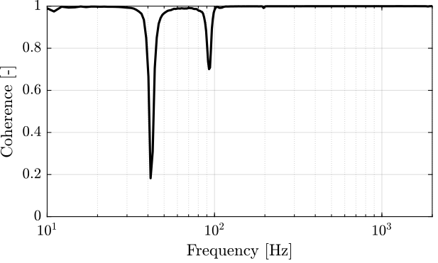
Figure 75: Obtained coherence for the IFF plant
Then the FRF are estimated and shown in Figure 76
%% Compute FRF function from Va to da
[frf_sweep, ~]    = tfestimate(leg_enc_sweep.Va,    leg_enc_sweep.Vs,    win, [], [], 1/Ts);
[frf_noise_hf, ~] = tfestimate(leg_enc_noise_hf.Va, leg_enc_noise_hf.Vs, win, [], [], 1/Ts);

%% Combine the FRF
iff_with_enc_frf = [frf_sweep(i_lf); frf_noise_hf(i_hf)];

Figure 76: Identified IFF Plant
Let’s now compare the IFF plants whether the encoders are fixed to the APA or not (Figure 77).
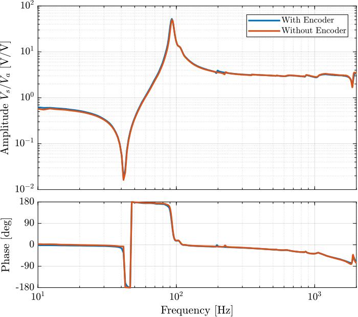
Figure 77: Effect of the encoder on the IFF plant
The transfer function from the excitation voltage \(V_a\) to the generated voltage \(V_s\) by the sensor stack is not influence by the fixation of the encoder. This means that the IFF control strategy should be as effective whether or not the encoders are fixed to the struts.
5.2 Comparison of all the Struts
Now all struts are measured using the same procedure and test bench as in Section 5.1.
5.2.1 FRF Identification - Setup
The identification of the struts dynamics is performed in two steps:
- The excitation signal is a white noise with small amplitude. This is used to estimate the low frequency dynamics.
- Then a high frequency noise band-passed between 300Hz and 2kHz is used to estimate the high frequency dynamics.
Then, the result of the first identification is used between 10Hz and 350Hz and the result of the second identification if used between 350Hz and 2kHz.
Here are the leg numbers that have been measured.
%% Numnbers of the measured legs
leg_nums = [1 2 3 4 5];
The data are loaded for both the first and second identification:
%% First identification (low frequency noise)
leg_noise = {};
for i = 1:length(leg_nums)
    leg_noise(i) = {load(sprintf('frf_data_leg_coder_%i_noise.mat', leg_nums(i)), 't', 'Va', 'Vs', 'de', 'da')};
end

%% Second identification (high frequency noise)
leg_noise_hf = {};
for i = 1:length(leg_nums)
    leg_noise_hf(i) = {load(sprintf('frf_data_leg_coder_%i_noise_hf.mat', leg_nums(i)), 't', 'Va', 'Vs', 'de', 'da')};
end
The time is the same for all measurements.
%% Time vector
t = leg_noise{1}.t - leg_noise{1}.t(1) ; % Time vector [s]

%% Sampling
Ts = (t(end) - t(1))/(length(t)-1); % Sampling Time [s]
Fs = 1/Ts; % Sampling Frequency [Hz]
Then we defined a “Hanning” windows that will be used for the spectral analysis:
win = hanning(ceil(0.5*Fs)); % Hannning Windows
We get the frequency vector that will be the same for all the frequency domain analysis.
% Only used to have the frequency vector "f"
[~, f] = tfestimate(leg_noise{1}.Va, leg_noise{1}.de, win, [], [], 1/Ts);
i_lf = f <= 350;
i_hf = f >  350;
5.2.2 FRF Identification - Encoder
In this section, the dynamics from \(V_a\) to \(d_e\) (encoder) is identified.
The coherence is computed and shown in Figure 78 for all the measured struts.
%% Coherence computation
coh_enc = zeros(length(f), length(leg_nums));
for i = 1:length(leg_nums)
    [coh_lf, ~] = mscohere(leg_noise{i}.Va,    leg_noise{i}.de,    win, [], [], 1/Ts);
    [coh_hf, ~] = mscohere(leg_noise_hf{i}.Va, leg_noise_hf{i}.de, win, [], [], 1/Ts);
    coh_enc(:, i) = [coh_lf(i_lf); coh_hf(i_hf)];
end
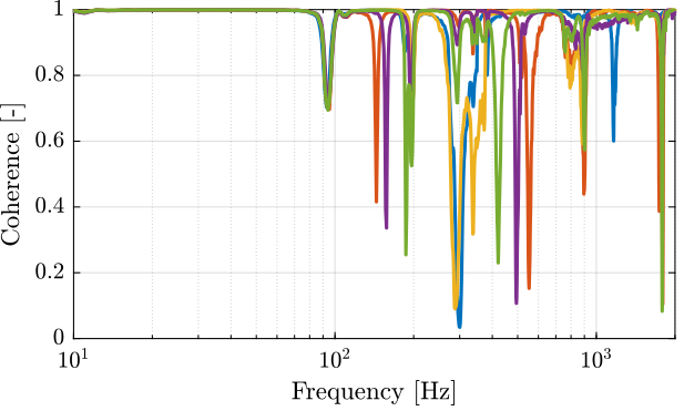
Figure 78: Obtained coherence for the plant from \(V_a\) to \(d_e\)
Then, the transfer function from the DAC output voltage \(V_a\) to the measured displacement by the encoder \(d_e\) is computed:
%% Transfer function estimation
enc_frf = zeros(length(f), length(leg_nums));

for i = 1:length(leg_nums)
    [frf_lf, ~] = tfestimate(leg_noise{i}.Va,    leg_noise{i}.de,    win, [], [], 1/Ts);
    [frf_hf, ~] = tfestimate(leg_noise_hf{i}.Va, leg_noise_hf{i}.de, win, [], [], 1/Ts);
    enc_frf(:, i) = [frf_lf(i_lf); frf_hf(i_hf)];
end
The obtained transfer functions are shown in Figure 79.
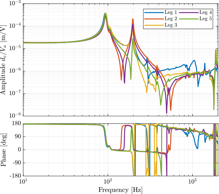
Figure 79: Estimated FRF for the DVF plant (transfer function from \(V_a\) to the encoder \(d_e\))
There is a very large variability of the dynamics as measured by the encoder as shown in Figure 79. Even-though the same peaks are seen for all of the struts (95Hz, 200Hz, 300Hz, 400Hz), the amplitude of the peaks are not the same. Moreover, the location or even the presence of complex conjugate zeros is changing from one strut to the other.
All of this will be explained in Section 6 thanks to the Simscape model.
5.2.3 FRF Identification - Interferometer
In this section, the dynamics from \(V_a\) to \(d_a\) (interferometer) is identified.
The coherence is computed and shown in Figure 80.
%% Coherence computation
coh_int = zeros(length(f), length(leg_nums));
for i = 1:length(leg_nums)
    [coh_lf, ~] = mscohere(leg_noise{i}.Va,    leg_noise{i}.da,    win, [], [], 1/Ts);
    [coh_hf, ~] = mscohere(leg_noise_hf{i}.Va, leg_noise_hf{i}.da, win, [], [], 1/Ts);
    coh_int(:, i) = [coh_lf(i_lf); coh_hf(i_hf)];
end
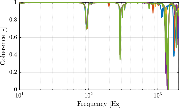
Figure 80: Obtained coherence for the plant from \(V_a\) to \(d_e\)
Then, the transfer function from the DAC output voltage \(V_a\) to the measured displacement by the Attocube is computed for all the struts and shown in Figure 81. All the struts are giving very similar FRF.
%% Transfer function estimation
int_frf = zeros(length(f), length(leg_nums));
for i = 1:length(leg_nums)
    [frf_lf, ~] = tfestimate(leg_noise{i}.Va,    leg_noise{i}.da,    win, [], [], 1/Ts);
    [frf_hf, ~] = tfestimate(leg_noise_hf{i}.Va, leg_noise_hf{i}.da, win, [], [], 1/Ts);
    int_frf(:, i) = [frf_lf(i_lf); frf_hf(i_hf)];
end
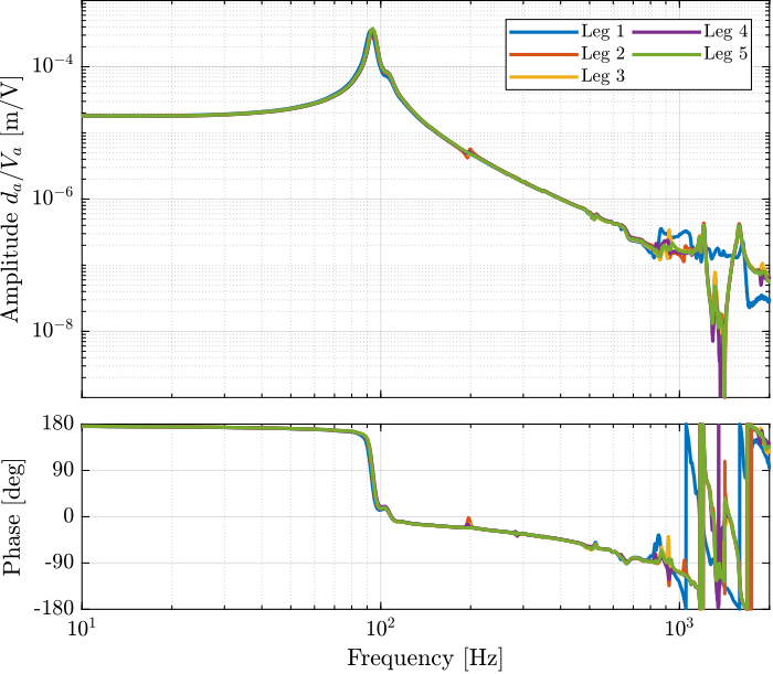
Figure 81: Estimated FRF for the DVF plant (transfer function from \(V_a\) to the encoder \(d_e\))
5.2.4 FRF Identification - Force Sensor
In this section, the dynamics from \(V_a\) to \(V_s\) is identified.
First the coherence is computed and shown in Figure 82.
%% Coherence
coh_iff = zeros(length(f), length(leg_nums));
for i = 1:length(leg_nums)
    [coh_lf, ~] = mscohere(leg_noise{i}.Va,    leg_noise{i}.Vs,    win, [], [], 1/Ts);
    [coh_hf, ~] = mscohere(leg_noise_hf{i}.Va, leg_noise_hf{i}.Vs, win, [], [], 1/Ts);
    coh_iff(:, i) = [coh_lf(i_lf); coh_hf(i_hf)];
end
Figure 82: Obtained coherence for the IFF plant
Then the FRF are estimated and shown in Figure 83. They are also shown all to be very similar.
%% FRF estimation of the transfer function from Va to Vs
iff_frf = zeros(length(f), length(leg_nums));
for i = 1:length(leg_nums)
    [frf_lf, ~] = tfestimate(leg_noise{i}.Va,    leg_noise{i}.Vs,    win, [], [], 1/Ts);
    [frf_hf, ~] = tfestimate(leg_noise_hf{i}.Va, leg_noise_hf{i}.Vs, win, [], [], 1/Ts);
    iff_frf(:, i) = [frf_lf(i_lf); frf_hf(i_hf)];
end
Figure 83: Identified IFF Plant
5.2.5 Conclusion
All the struts are giving very consistent behavior from the excitation voltage \(V_a\) to the force sensor generated voltage \(V_s\) and to the interferometer measured displacement \(d_a\). However, the dynamics from \(V_a\) to the encoder measurement \(d_e\) is much more complex and variable from one strut to the other.
The measured FRF are now saved for further use.
%% Save the estimated FRF for further analysis
save('mat/meas_struts_frf.mat', 'f', 'Ts', 'enc_frf', 'int_frf', 'iff_frf', 'leg_nums');
6 Test Bench Struts - Simscape Model
The same simscape model that was presented in Section 4 is here used. However, now the full strut is put instead of only the APA (see Figure 84).
Figure 84: Screenshot of the Simscape model of the strut fixed to the bench
This Simscape model is used to:
- compare the measured FRF with the modelled FRF
- help the correct understanding/interpretation of the results
- tune the model of the struts (APA, flexible joints, encoder)
This study is structured as follow:
- Section 6.1: the measured FRF are compared with the 2DoF APA model.
- Section 6.2: the flexible APA model is used, and the effect of a misalignment of the APA and flexible joints is studied. It is found that the misalignment has a large impact on the dynamics from \(V_a\) to \(d_e\).
- Section 6.3: the effect of the flexible joint’s stiffness on the dynamics is studied. It is found that the axial stiffness of the joints has a large impact on the location of the zeros on the transfer function from \(V_s\) to \(d_e\).
6.1 Comparison with the 2-DoF Model
6.1.1 First Identification
The strut is initialized with default parameters (optimized parameters identified from previous experiments).
%% Initialize structure containing data for the Simscape model
n_hexapod = struct();
n_hexapod.flex_bot = initializeBotFlexibleJoint('type', '4dof');
n_hexapod.flex_top = initializeTopFlexibleJoint('type', '4dof');
n_hexapod.actuator = initializeAPA('type', '2dof');
The inputs and outputs of the model are defined.
%% Input/Output definition
clear io; io_i = 1;
io(io_i) = linio([mdl, '/Va'], 1, 'openinput');  io_i = io_i + 1; % Actuator Voltage
io(io_i) = linio([mdl, '/Vs'], 1, 'openoutput'); io_i = io_i + 1; % Sensor Voltage
io(io_i) = linio([mdl, '/de'], 1, 'openoutput'); io_i = io_i + 1; % Encoder
io(io_i) = linio([mdl, '/da'], 1, 'openoutput'); io_i = io_i + 1; % Interferometer
The dynamics is identified and shown in Figure 85.
%% Run the linearization
Gs = linearize(mdl, io, 0.0, options);
Gs.InputName  = {'Va'};
Gs.OutputName = {'Vs', 'de', 'da'};
Figure 85: Identified transfer function from \(V_a\) to \(V_s\) and from \(V_a\) to \(d_e,d_a\) using the simple 2DoF model for the APA
6.1.2 Comparison with the experimental Data
The experimentally measured FRF are loaded.
%% Load measured FRF
load('meas_struts_frf.mat', 'f', 'Ts', 'enc_frf', 'int_frf', 'iff_frf', 'leg_nums');
%% Add time delay to the Simscape model
Gs = exp(-s*Ts)*Gs;
The FRF from \(V_a\) to \(d_a\) as well as from \(V_a\) to \(V_s\) are shown in Figure 86 and compared with the model. They are both found to match quite well with the model.
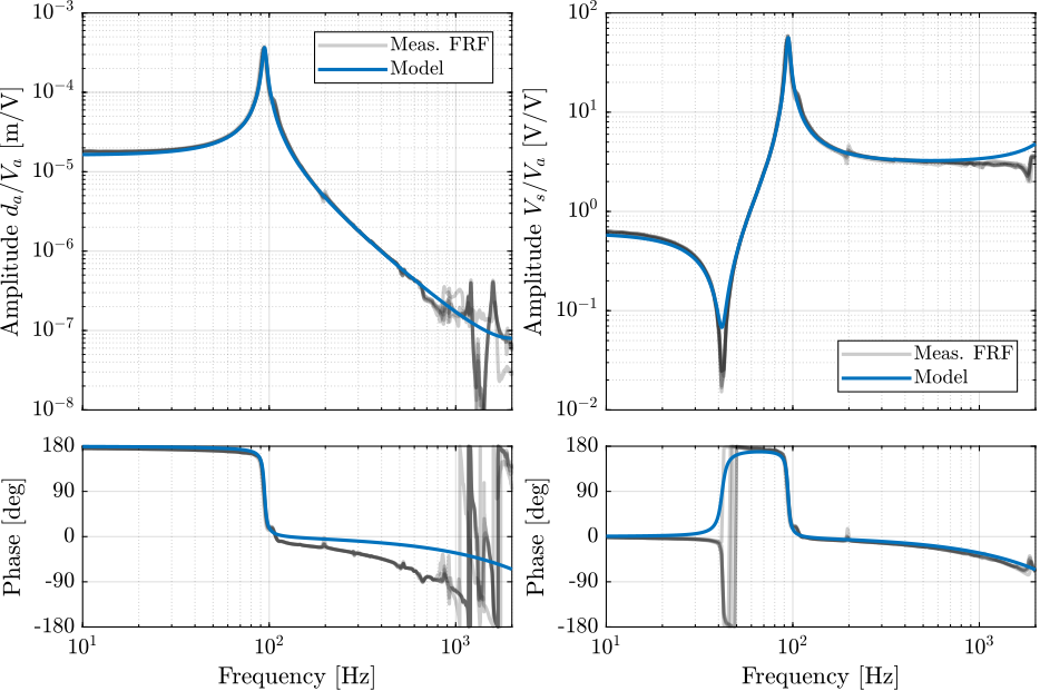
Figure 86: Comparison of the measured FRF and the optimized model
The measured FRF from \(V_a\) to \(d_e\) (encoder) is compared with the model in Figure 87.
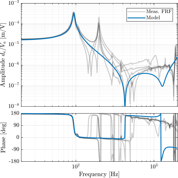
Figure 87: Comparison of the measured FRF and the optimized model
The 2-DoF model is quite effective in modelling the transfer function from actuator to force sensor and from actuator to interferometer (Figure 86). But it is not effective in modeling the transfer function from actuator to encoder (Figure 87). This is due to the fact that resonances greatly affecting the encoder reading are not modelled. In the next section, flexible model of the APA will be used to model such resonances.
6.2 Effect of a misalignment of the APA and flexible joints on the transfer function from actuator to encoder
As shown in Figure 79, the dynamics from actuator to encoder for all the struts is very different.
This could be explained by a large variability in the alignment of the flexible joints and the APA (at the time, the alignment pins were not used).
Depending on the alignment, the spurious resonances of the struts (Figure 88) can be excited differently.
Figure 88: Spurious resonances. a) X-bending mode at 189Hz. b) Y-bending mode at 285Hz. c) Z-torsion mode at 400Hz
For instance, consider Figure 89 where there is a misalignment in the \(y\) direction. In such case, the mode at 200Hz is foreseen to be more excited as the misalignment \(d_y\) increases and therefore the dynamics from the actuator to the encoder should also change around 200Hz.
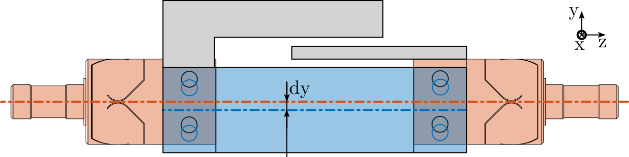
Figure 89: Mis-alignement between the joints and the APA
If the misalignment is in the \(x\) direction, the mode at 285Hz should be more affected whereas a misalignment in the \(z\) direction should not affect these resonances.
Such statement is studied in this section.
But first, the measured FRF of the struts are loaded.
%% Load measured FRF of the struts
load('meas_struts_frf.mat', 'f', 'Ts', 'enc_frf', 'int_frf', 'iff_frf', 'leg_nums');
6.2.1 Perfectly aligned APA
Let’s first consider that the strut is perfectly mounted such that the two flexible joints and the APA are aligned.
%% Initialize Simscape data
n_hexapod.flex_bot = initializeBotFlexibleJoint('type', '4dof');
n_hexapod.flex_top = initializeTopFlexibleJoint('type', '4dof');
n_hexapod.actuator = initializeAPA('type', 'flexible');
And define the inputs and outputs of the models:
- Input: voltage generated by the DAC
- Output: measured displacement by the encoder
%% Input/Output definition
clear io; io_i = 1;
io(io_i) = linio([mdl, '/Va'],  1, 'openinput');  io_i = io_i + 1; % Actuator Voltage
io(io_i) = linio([mdl, '/de'],  1, 'openoutput'); io_i = io_i + 1; % Encoder
The transfer function is identified and shown in Figure 90.
%% Identification
Gs = exp(-s*Ts)*linearize(mdl, io, 0.0, options);
Gs.InputName  = {'Va'};
Gs.OutputName = {'de'};
From Figure 90, it is clear that:
- The model with perfect alignment is not matching the measured FRF
- The mode at 200Hz is not present in the identified dynamics of the Simscape model
- The measured FRF have different shapes
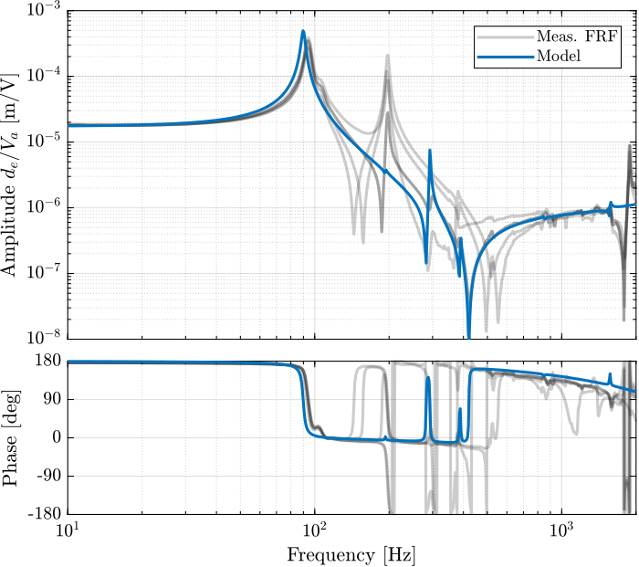
Figure 90: Comparison of the model with a perfectly aligned APA and flexible joints with the measured FRF from actuator to encoder
Why is the flexible mode of the strut at 200Hz is not seen in the model in Figure 90?
Probably because the presence of this mode is not due because of the “unbalanced” mass of the encoder, but rather because of the misalignment of the APA with respect to the two flexible joints. This will be verified in the next sections.
6.2.2 Effect of a misalignment in y
Let’s compute the transfer function from output DAC voltage \(V_s\) to the measured displacement by the encoder \(d_e\) for several misalignment in the \(y\) direction:
%% Considered misalignments
dy_aligns = [-0.5, -0.1, 0, 0.1, 0.5]*1e-3; % [m]
%% Transfer functions from u to de for all the misalignment in y direction
Gs_align = {zeros(length(dy_aligns), 1)};

for i = 1:length(dy_aligns)
    n_hexapod.actuator = initializeAPA('type', 'flexible', 'd_align', [0; dy_aligns(i); 0]);

    G = exp(-s*Ts)*linearize(mdl, io, 0.0, options);
    G.InputName  = {'Va'};
    G.OutputName = {'de'};

    Gs_align(i) = {G};
end
The obtained dynamics are shown in Figure 91.
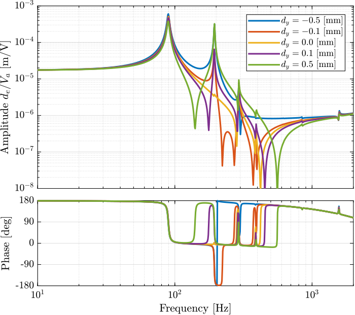
Figure 91: Effect of a misalignement in the \(y\) direction
The alignment of the APA with the flexible joints as a huge influence on the dynamics from actuator voltage to measured displacement by the encoder. The misalignment in the \(y\) direction mostly influences:
- the presence of the flexible mode at 200Hz
- the location of the complex conjugate zero between the first two resonances:
- if \(d_y < 0\): there is no zero between the two resonances and possibly not even between the second and third ones
- if \(d_y > 0\): there is a complex conjugate zero between the first two resonances
- the location of the high frequency complex conjugate zeros at 500Hz (secondary effect, as the axial stiffness of the joint also has large effect on the position of this zero)
6.2.3 Effect of a misalignment in x
Let’s compute the transfer function from output DAC voltage to the measured displacement by the encoder for several misalignment in the \(x\) direction:
%% Considered misalignments
dx_aligns = [-0.1, -0.05, 0, 0.05, 0.1]*1e-3; % [m]
%% Transfer functions from u to de for all the misalignment in x direction
Gs_align = {zeros(length(dx_aligns), 1)};

for i = 1:length(dx_aligns)
    n_hexapod.actuator = initializeAPA('type', 'flexible', 'd_align', [dx_aligns(i); 0; 0]);

    G = exp(-s*Ts)*linearize(mdl, io, 0.0, options);
    G.InputName  = {'Va'};
    G.OutputName = {'de'};

    Gs_align(i) = {G};
end
The obtained dynamics are shown in Figure 92.
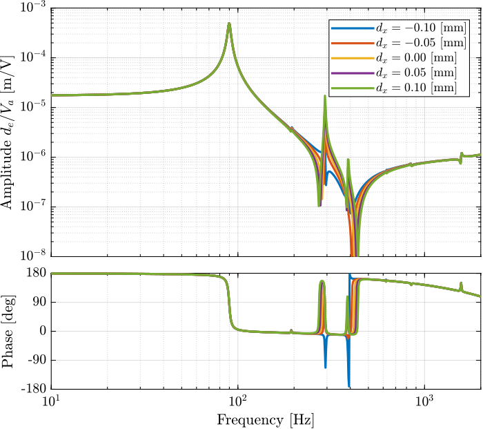
Figure 92: Effect of a misalignement in the \(x\) direction
The misalignment in the \(x\) direction mostly influences the presence of the flexible mode at 300Hz.
6.2.4 Find the misalignment of each strut
From the previous analysis on the effect of a \(x\) and \(y\) misalignment, it is possible to estimate the \(x,y\) misalignment of the measured struts.
The misalignment that gives the best match for the FRF are defined below.
%% Tuned misalignment [m]
d_aligns = [[-0.05,  -0.3,  0];
            [ 0,      0.5,  0];
            [-0.1,   -0.3,  0];
            [ 0,      0.3,  0];
            [-0.05,   0.05, 0]]'*1e-3;
For each misalignment, the dynamics from the DAC voltage to the encoder measurement is identified.
%% Idenfity the transfer function from actuator to encoder for all cases
Gs_align = {zeros(size(d_aligns,2), 1)};

for i = 1:size(d_aligns,2)
    n_hexapod.actuator = initializeAPA('type', 'flexible', 'd_align', d_aligns(:,i));

    G = exp(-s*Ts)*linearize(mdl, io, 0.0, options);
    G.InputName  = {'Va'};
    G.OutputName = {'de'};

    Gs_align(i) = {G};
end
The results are shown in Figure 93.
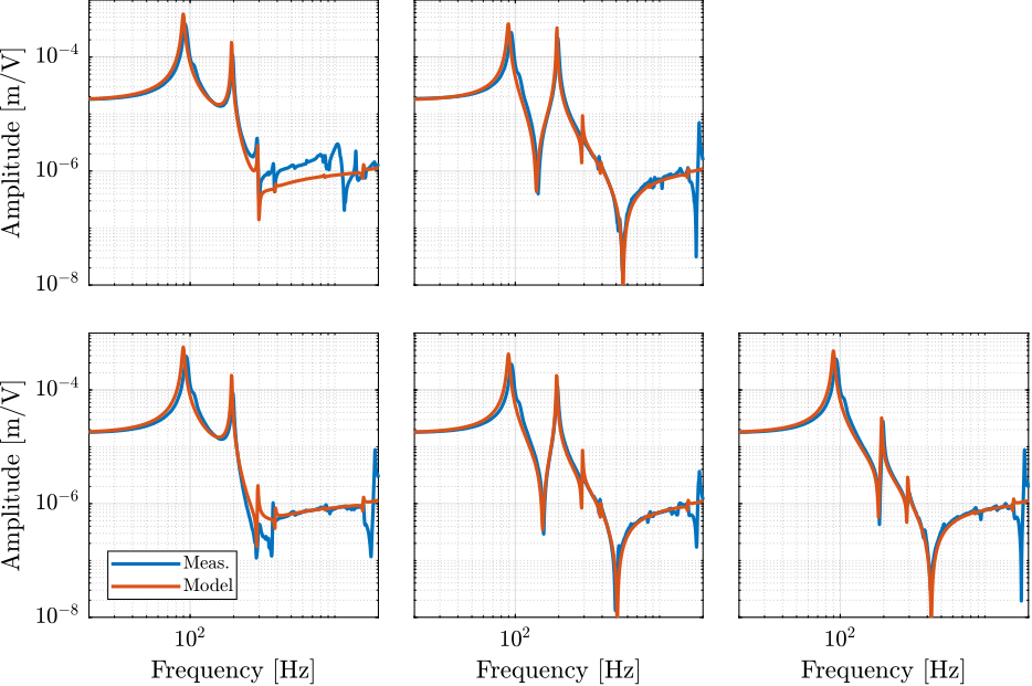
Figure 93: Comparison (model and measurements) of the FRF from DAC voltage u to measured displacement by the encoders for all the struts
By tuning the misalignment of the APA with respect to the flexible joints, it is possible to obtain a good fit between the model and the measurements (Figure 93).
If encoders are to be used when fixed on the struts, it is therefore very important to properly align the APA and the flexible joints when mounting the struts.
In the future, a “pin” will be used to better align the APA with the flexible joints. We can expect the amplitude of the spurious resonances to decrease.
6.3 Effect of flexible joint’s stiffness
As the struts are composed of one APA and two flexible joints, it is obvious that the flexible joint characteristics will change the dynamic behavior of the struts.
Using the Simscape model, the effect of the flexible joint’s characteristics on the dynamics as measured on the test bench are studied:
- Section 6.3.1: the effects of a change of bending stiffness is studied
- Section 6.3.2: the effects of a change of axial stiffness is studied
- Section 6.3.3: the effects of a change of bending damping is studied
The studied dynamics is between \(V_a\) and the encoder displacement \(d_e\).
%% Input/Output definition
clear io; io_i = 1;
io(io_i) = linio([mdl, '/Va'],  1, 'openinput');  io_i = io_i + 1; % Actuator Voltage
io(io_i) = linio([mdl, '/de'],  1, 'openoutput'); io_i = io_i + 1; % Encoder
6.3.1 Effect of bending stiffness of the flexible joints
Let’s initialize an APA which is a little bit misaligned.
%% APA Initialization
n_hexapod.actuator = initializeAPA('type', 'flexible', 'd_align', [0.1e-3; 0.5e-3; 0]);
The bending stiffnesses for which the dynamics is identified are defined below.
%% Tested bending stiffnesses [Nm/rad]
kRs = [3, 4, 5, 6, 7];
Then the identification is performed for all the values of the bending stiffnesses.
%% Idenfity the transfer function from actuator to encoder for all bending stiffnesses
Gs = {zeros(length(kRs), 1)};

for i = 1:length(kRs)
    n_hexapod.flex_bot = initializeBotFlexibleJoint(...
        'type', '4dof', ...
        'kRx', kRs(i), ...
        'kRy', kRs(i));
    n_hexapod.flex_top = initializeTopFlexibleJoint(...
        'type', '4dof', ...
        'kRx', kRs(i), ...
        'kRy', kRs(i));

    G = exp(-s*Ts)*linearize(mdl, io, 0.0, options);
    G.InputName  = {'Va'};
    G.OutputName = {'de'};

    Gs(i) = {G};
end
The obtained dynamics from DAC voltage to encoder measurements are compared in Figure 94.
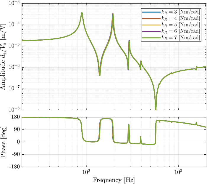
Figure 94: Dynamics from DAC output to encoder for several bending stiffnesses
The bending stiffness of the joints has little impact on the transfer function from \(V_a\) to \(d_e\).
6.3.2 Effect of axial stiffness of the flexible joints
The axial stiffnesses for which the dynamics is identified are defined below.
%% Tested axial stiffnesses [N/m]
kzs = [5e7 7.5e7 1e8 2.5e8];
Then the identification is performed for all the values of the bending stiffnesses.
%% Idenfity the transfer function from actuator to encoder for all bending stiffnesses
Gs = {zeros(length(kzs), 1)};

for i = 1:length(kzs)
    n_hexapod.flex_bot = initializeBotFlexibleJoint(...
        'type', '4dof', ...
        'kz', kzs(i));
    n_hexapod.flex_top = initializeTopFlexibleJoint(...
        'type', '4dof', ...
        'kz', kzs(i));

    G = exp(-s*Ts)*linearize(mdl, io, 0.0, options);
    G.InputName  = {'Va'};
    G.OutputName = {'de'};

    Gs(i) = {G};
end
The obtained dynamics from DAC voltage to encoder measurements are compared in Figure 95.
Figure 95: Dynamics from DAC output to encoder for several axial stiffnesses
The axial stiffness of the flexible joint has a large impact on the frequency of the complex conjugate zero. Using the measured FRF on the test-bench, if is therefore possible to estimate the axial stiffness of the flexible joints from the location of the zero.
This method gives nice match between the measured FRF and the one extracted from the simscape model, however it could give not so accurate values of the joint’s axial stiffness as other factors are also influencing the location of the zero.
Using this method, an axial stiffness of \(70 N/\mu m\) is found to give good results (and is reasonable based on the finite element models).
6.3.3 Effect of bending damping
Now let’s study the effect of the bending damping of the flexible joints.
The tested bending damping are defined below:
%% Tested bending dampings [Nm/(rad/s)]
cRs = [1e-3, 5e-3, 1e-2, 5e-2, 1e-1];
Then the identification is performed for all the values of the bending damping.
%% Idenfity the transfer function from actuator to encoder for all bending dampins
Gs = {zeros(length(kRs), 1)};

for i = 1:length(kRs)
    n_hexapod.flex_bot = initializeBotFlexibleJoint(...
        'type', '4dof', ...
        'cRx', cRs(i), ...
        'cRy', cRs(i));
    n_hexapod.flex_top = initializeTopFlexibleJoint(...
        'type', '4dof', ...
        'cRx', cRs(i), ...
        'cRy', cRs(i));

    G = exp(-s*Ts)*linearize(mdl, io, 0.0, options);
    G.InputName  = {'Va'};
    G.OutputName = {'de'};

    Gs(i) = {G};
end
The results are shown in Figure 96.
Figure 96: Dynamics from DAC output to encoder for several bending damping
Adding damping in bending for the flexible joints could be a nice way to reduce the effects of the spurious resonances of the struts.
How to effectively add damping to the flexible joints?
One idea would be to introduce a sheet of damping material inside the flexible joint. Not sure is would be effect though.
7 Function
7.1 initializeBotFlexibleJoint - Initialize Flexible Joint
Function description
function [flex_bot] = initializeBotFlexibleJoint(args)
% initializeBotFlexibleJoint -
%
% Syntax: [flex_bot] = initializeBotFlexibleJoint(args)
%
% Inputs:
%    - args -
%
% Outputs:
%    - flex_bot -
Optional Parameters
arguments
    args.type      char   {mustBeMember(args.type,{'2dof', '3dof', '4dof'})} = '2dof'

    args.kRx (6,1) double {mustBeNumeric, mustBePositive} = ones(6,1)*5
    args.kRy (6,1) double {mustBeNumeric, mustBePositive} = ones(6,1)*5
    args.kRz (6,1) double {mustBeNumeric, mustBePositive} = ones(6,1)*260
    args.kz  (6,1) double {mustBeNumeric, mustBePositive} = ones(6,1)*7e7

    args.cRx (6,1) double {mustBeNumeric, mustBePositive} = ones(6,1)*0.001
    args.cRy (6,1) double {mustBeNumeric, mustBePositive} = ones(6,1)*0.001
    args.cRz (6,1) double {mustBeNumeric, mustBePositive} = ones(6,1)*0.001
    args.cz  (6,1) double {mustBeNumeric, mustBePositive} = ones(6,1)*0.001
end
Initialize the structure
flex_bot = struct();
Set the Joint’s type
switch args.type
  case '2dof'
    flex_bot.type = 1;
  case '3dof'
    flex_bot.type = 2;
  case '4dof'
    flex_bot.type = 3;
end
Set parameters
flex_bot.kRx = args.kRx;
flex_bot.kRy = args.kRy;
flex_bot.kRz = args.kRz;
flex_bot.kz  = args.kz;
flex_bot.cRx = args.cRx;
flex_bot.cRy = args.cRy;
flex_bot.cRz = args.cRz;
flex_bot.cz  = args.cz;
7.2 initializeTopFlexibleJoint - Initialize Flexible Joint
Function description
function [flex_top] = initializeTopFlexibleJoint(args)
% initializeTopFlexibleJoint -
%
% Syntax: [flex_top] = initializeTopFlexibleJoint(args)
%
% Inputs:
%    - args -
%
% Outputs:
%    - flex_top -
Optional Parameters
arguments
    args.type      char   {mustBeMember(args.type,{'2dof', '3dof', '4dof'})} = '2dof'

    args.kRx (6,1) double {mustBeNumeric, mustBePositive} = ones(6,1)*5
    args.kRy (6,1) double {mustBeNumeric, mustBePositive} = ones(6,1)*5
    args.kRz (6,1) double {mustBeNumeric, mustBePositive} = ones(6,1)*260
    args.kz  (6,1) double {mustBeNumeric, mustBePositive} = ones(6,1)*7e7

    args.cRx (6,1) double {mustBeNumeric, mustBePositive} = ones(6,1)*0.001
    args.cRy (6,1) double {mustBeNumeric, mustBePositive} = ones(6,1)*0.001
    args.cRz (6,1) double {mustBeNumeric, mustBePositive} = ones(6,1)*0.001
    args.cz  (6,1) double {mustBeNumeric, mustBePositive} = ones(6,1)*0.001
end
Initialize the structure
flex_top = struct();
Set the Joint’s type
switch args.type
  case '2dof'
    flex_top.type = 1;
  case '3dof'
    flex_top.type = 2;
  case '4dof'
    flex_top.type = 3;
end
Set parameters
flex_top.kRx = args.kRx;
flex_top.kRy = args.kRy;
flex_top.kRz = args.kRz;
flex_top.kz  = args.kz;
flex_top.cRx = args.cRx;
flex_top.cRy = args.cRy;
flex_top.cRz = args.cRz;
flex_top.cz  = args.cz;
7.3 initializeAPA - Initialize APA
Function description
function [actuator] = initializeAPA(args)
% initializeAPA -
%
% Syntax: [actuator] = initializeAPA(args)
%
% Inputs:
%    - args -
%
% Outputs:
%    - actuator -
Optional Parameters
arguments
    args.type      char   {mustBeMember(args.type,{'2dof', 'flexible frame', 'flexible'})} = '2dof'

    % Actuator and Sensor constants
    args.Ga  (1,1) double {mustBeNumeric} = 0
    args.Gs  (1,1) double {mustBeNumeric} = 0

    % For 2DoF
    args.k   (6,1) double {mustBeNumeric, mustBePositive} = ones(6,1)*0.38e6
    args.ke  (6,1) double {mustBeNumeric, mustBePositive} = ones(6,1)*1.75e6
    args.ka  (6,1) double {mustBeNumeric, mustBePositive} = ones(6,1)*3e7

    args.c   (6,1) double {mustBeNumeric, mustBePositive} = ones(6,1)*3e1
    args.ce  (6,1) double {mustBeNumeric, mustBePositive} = ones(6,1)*2e1
    args.ca  (6,1) double {mustBeNumeric, mustBePositive} = ones(6,1)*2e1

    args.Leq (6,1) double {mustBeNumeric} = ones(6,1)*0.056

    % Force Flexible APA
    args.xi (1,1) double {mustBeNumeric, mustBePositive} = 0.01
    args.d_align (3,1) double {mustBeNumeric} = zeros(3,1) % [m]

    % For Flexible Frame
    args.ks (1,1) double {mustBeNumeric, mustBePositive} = 235e6
    args.cs (1,1) double {mustBeNumeric, mustBePositive} = 1e1
end
Initialize Structure
actuator = struct();
Type
switch args.type
  case '2dof'
    actuator.type = 1;
  case 'flexible frame'
    actuator.type = 2;
  case 'flexible'
    actuator.type = 3;
end
Actuator/Sensor Constants
if args.Ga == 0
    switch args.type
      case '2dof'
        actuator.Ga = -30.0;
      case 'flexible frame'
        actuator.Ga = 1; % TODO
      case 'flexible'
        actuator.Ga = 23.4;
    end
else
    actuator.Ga = args.Ga; % Actuator gain [N/V]
end
if args.Gs == 0
    switch args.type
      case '2dof'
        actuator.Gs = 0.098;
      case 'flexible frame'
        actuator.Gs = 1; % TODO
      case 'flexible'
        actuator.Gs = -4674824;
    end
else
    actuator.Gs = args.Gs; % Sensor gain [V/m]
end
2DoF parameters
actuator.k  = args.k;  % [N/m]
actuator.ke = args.ke; % [N/m]
actuator.ka = args.ka; % [N/m]

actuator.c  = args.c;  % [N/(m/s)]
actuator.ce = args.ce; % [N/(m/s)]
actuator.ca = args.ca; % [N/(m/s)]

actuator.Leq = args.Leq; % [m]
Flexible frame and fully flexible
switch args.type
  case 'flexible frame'
    actuator.K = readmatrix('APA300ML_b_mat_K.CSV'); % Stiffness Matrix
    actuator.M = readmatrix('APA300ML_b_mat_M.CSV'); % Mass Matrix
    actuator.P = extractNodes('APA300ML_b_out_nodes_3D.txt'); % Node coordinates [m]
  case 'flexible'
    actuator.K = readmatrix('full_APA300ML_K.CSV'); % Stiffness Matrix
    actuator.M = readmatrix('full_APA300ML_M.CSV'); % Mass Matrix
    actuator.P = extractNodes('full_APA300ML_out_nodes_3D.txt'); % Node coordiantes [m]
    actuator.d_align = args.d_align;
end

actuator.xi = args.xi; % Damping ratio

actuator.ks = args.ks; % Stiffness of one stack [N/m]
actuator.cs = args.cs; % Damping of one stack [N/m]
7.4 generateSweepExc: Generate sweep sinus excitation
Function description
function [U_exc] = generateSweepExc(args)
% generateSweepExc - Generate a Sweep Sine excitation signal
%
% Syntax: [U_exc] = generateSweepExc(args)
%
% Inputs:
%    - args - Optinal arguments:
%        - Ts              - Sampling Time                                              - [s]
%        - f_start         - Start frequency of the sweep                               - [Hz]
%        - f_end           - End frequency of the sweep                                 - [Hz]
%        - V_mean          - Mean value of the excitation voltage                       - [V]
%        - V_exc           - Excitation Amplitude for the Sweep, could be numeric or TF - [V]
%        - t_start         - Time at which the sweep begins                             - [s]
%        - exc_duration    - Duration of the sweep                                      - [s]
%        - sweep_type      - 'logarithmic' or 'linear'                                  - [-]
%        - smooth_ends     - 'true' or 'false': smooth transition between 0 and V_mean  - [-]
Optional Parameters
arguments
    args.Ts              (1,1) double  {mustBeNumeric, mustBePositive} = 1e-4
    args.f_start         (1,1) double  {mustBeNumeric, mustBePositive} = 1
    args.f_end           (1,1) double  {mustBeNumeric, mustBePositive} = 1e3
    args.V_mean          (1,1) double  {mustBeNumeric} = 0
    args.V_exc                                         = 1
    args.t_start         (1,1) double  {mustBeNumeric, mustBeNonnegative} = 5
    args.exc_duration    (1,1) double  {mustBeNumeric, mustBePositive} = 10
    args.sweep_type            char    {mustBeMember(args.sweep_type,{'log', 'lin'})} = 'lin'
    args.smooth_ends           logical {mustBeNumericOrLogical} = true
end
Sweep Sine part
t_sweep = 0:args.Ts:args.exc_duration;

if strcmp(args.sweep_type, 'log')
    V_exc = sin(2*pi*args.f_start * args.exc_duration/log(args.f_end/args.f_start) * (exp(log(args.f_end/args.f_start)*t_sweep/args.exc_duration) - 1));
elseif strcmp(args.sweep_type, 'lin')
    V_exc = sin(2*pi*(args.f_start + (args.f_end - args.f_start)/2/args.exc_duration*t_sweep).*t_sweep);
else
    error('sweep_type should either be equal to "log" or to "lin"');
end
if isnumeric(args.V_exc)
    V_sweep = args.V_mean + args.V_exc*V_exc;
elseif isct(args.V_exc)
    if strcmp(args.sweep_type, 'log')
        V_sweep = args.V_mean + abs(squeeze(freqresp(args.V_exc, args.f_start*(args.f_end/args.f_start).^(t_sweep/args.exc_duration), 'Hz')))'.*V_exc;
    elseif strcmp(args.sweep_type, 'lin')
        V_sweep = args.V_mean + abs(squeeze(freqresp(args.V_exc, args.f_start+(args.f_end-args.f_start)/args.exc_duration*t_sweep, 'Hz')))'.*V_exc;
    end
end
Smooth Ends
if args.t_start > 0
    t_smooth_start = args.Ts:args.Ts:args.t_start;

    V_smooth_start = zeros(size(t_smooth_start));
    V_smooth_end   = zeros(size(t_smooth_start));

    if args.smooth_ends
        Vd_max = args.V_mean/(0.7*args.t_start);

        V_d = zeros(size(t_smooth_start));
        V_d(t_smooth_start < 0.2*args.t_start) = t_smooth_start(t_smooth_start < 0.2*args.t_start)*Vd_max/(0.2*args.t_start);
        V_d(t_smooth_start > 0.2*args.t_start & t_smooth_start < 0.7*args.t_start) = Vd_max;
        V_d(t_smooth_start > 0.7*args.t_start & t_smooth_start < 0.9*args.t_start) = Vd_max - (t_smooth_start(t_smooth_start > 0.7*args.t_start & t_smooth_start < 0.9*args.t_start) - 0.7*args.t_start)*Vd_max/(0.2*args.t_start);

        V_smooth_start = cumtrapz(V_d)*args.Ts;

        V_smooth_end = args.V_mean - V_smooth_start;
    end
else
    V_smooth_start = [];
    V_smooth_end = [];
end
Combine Excitation signals
V_exc = [V_smooth_start, V_sweep, V_smooth_end];
t_exc = args.Ts*[0:1:length(V_exc)-1];
U_exc = [t_exc; V_exc];
7.5 generateShapedNoise: Generate Shaped Noise excitation
Function description
function [U_exc] = generateShapedNoise(args)
% generateShapedNoise - Generate a Shaped Noise excitation signal
%
% Syntax: [U_exc] = generateShapedNoise(args)
%
% Inputs:
%    - args - Optinal arguments:
%        - Ts              - Sampling Time                                              - [s]
%        - V_mean          - Mean value of the excitation voltage                       - [V]
%        - V_exc           - Excitation Amplitude, could be numeric or TF               - [V rms]
%        - t_start         - Time at which the noise begins                             - [s]
%        - exc_duration    - Duration of the noise                                      - [s]
%        - smooth_ends     - 'true' or 'false': smooth transition between 0 and V_mean  - [-]
Optional Parameters
arguments
    args.Ts              (1,1) double  {mustBeNumeric, mustBePositive} = 1e-4
    args.V_mean          (1,1) double  {mustBeNumeric} = 0
    args.V_exc                                         = 1
    args.t_start         (1,1) double  {mustBeNumeric, mustBePositive} = 5
    args.exc_duration    (1,1) double  {mustBeNumeric, mustBePositive} = 10
    args.smooth_ends           logical {mustBeNumericOrLogical} = true
end
Shaped Noise
t_noise = 0:args.Ts:args.exc_duration;
if isnumeric(args.V_exc)
    V_noise = args.V_mean + args.V_exc*sqrt(1/args.Ts/2)*randn(length(t_noise), 1)';
elseif isct(args.V_exc)
    V_noise = args.V_mean + lsim(args.V_exc, sqrt(1/args.Ts/2)*randn(length(t_noise), 1), t_noise)';
end
Smooth Ends
t_smooth_start = args.Ts:args.Ts:args.t_start;

V_smooth_start = zeros(size(t_smooth_start));
V_smooth_end   = zeros(size(t_smooth_start));

if args.smooth_ends
    Vd_max = args.V_mean/(0.7*args.t_start);

    V_d = zeros(size(t_smooth_start));
    V_d(t_smooth_start < 0.2*args.t_start) = t_smooth_start(t_smooth_start < 0.2*args.t_start)*Vd_max/(0.2*args.t_start);
    V_d(t_smooth_start > 0.2*args.t_start & t_smooth_start < 0.7*args.t_start) = Vd_max;
    V_d(t_smooth_start > 0.7*args.t_start & t_smooth_start < 0.9*args.t_start) = Vd_max - (t_smooth_start(t_smooth_start > 0.7*args.t_start & t_smooth_start < 0.9*args.t_start) - 0.7*args.t_start)*Vd_max/(0.2*args.t_start);

    V_smooth_start = cumtrapz(V_d)*args.Ts;

    V_smooth_end = args.V_mean - V_smooth_start;
end
Combine Excitation signals
V_exc = [V_smooth_start, V_noise, V_smooth_end];
t_exc = args.Ts*[0:1:length(V_exc)-1];
U_exc = [t_exc; V_exc];
7.6 generateSinIncreasingAmpl: Generate Sinus with increasing amplitude
Function description
function [U_exc] = generateSinIncreasingAmpl(args)
% generateSinIncreasingAmpl - Generate Sinus with increasing amplitude
%
% Syntax: [U_exc] = generateSinIncreasingAmpl(args)
%
% Inputs:
%    - args - Optinal arguments:
%        - Ts              - Sampling Time                                              - [s]
%        - V_mean          - Mean value of the excitation voltage                       - [V]
%        - sin_ampls       - Excitation Amplitudes                                      - [V]
%        - sin_freq        - Excitation Frequency                                       - [Hz]
%        - sin_num         - Number of period for each amplitude                        - [-]
%        - t_start         - Time at which the excitation begins                        - [s]
%        - smooth_ends     - 'true' or 'false': smooth transition between 0 and V_mean  - [-]
Optional Parameters
arguments
    args.Ts              (1,1) double  {mustBeNumeric, mustBePositive} = 1e-4
    args.V_mean          (1,1) double  {mustBeNumeric} = 0
    args.sin_ampls             double  {mustBeNumeric, mustBePositive} = [0.1, 0.2, 0.3]
    args.sin_period      (1,1) double  {mustBeNumeric, mustBePositive} = 1
    args.sin_num         (1,1) double  {mustBeNumeric, mustBePositive, mustBeInteger} = 3
    args.t_start         (1,1) double  {mustBeNumeric, mustBePositive} = 5
    args.smooth_ends           logical {mustBeNumericOrLogical} = true
end
Sinus excitation
t_noise = 0:args.Ts:args.sin_period*args.sin_num;
sin_exc = [];
for sin_ampl = args.sin_ampls
    sin_exc = [sin_exc, args.V_mean + sin_ampl*sin(2*pi/args.sin_period*t_noise)];
end
Smooth Ends
t_smooth_start = args.Ts:args.Ts:args.t_start;

V_smooth_start = zeros(size(t_smooth_start));
V_smooth_end   = zeros(size(t_smooth_start));

if args.smooth_ends
    Vd_max = args.V_mean/(0.7*args.t_start);

    V_d = zeros(size(t_smooth_start));
    V_d(t_smooth_start < 0.2*args.t_start) = t_smooth_start(t_smooth_start < 0.2*args.t_start)*Vd_max/(0.2*args.t_start);
    V_d(t_smooth_start > 0.2*args.t_start & t_smooth_start < 0.7*args.t_start) = Vd_max;
    V_d(t_smooth_start > 0.7*args.t_start & t_smooth_start < 0.9*args.t_start) = Vd_max - (t_smooth_start(t_smooth_start > 0.7*args.t_start & t_smooth_start < 0.9*args.t_start) - 0.7*args.t_start)*Vd_max/(0.2*args.t_start);

    V_smooth_start = cumtrapz(V_d)*args.Ts;

    V_smooth_end = args.V_mean - V_smooth_start;
end
Combine Excitation signals
V_exc = [V_smooth_start, sin_exc, V_smooth_end];
t_exc = args.Ts*[0:1:length(V_exc)-1];
U_exc = [t_exc; V_exc];