Sensor Fusion - Test Bench

Table of ContentsClose

1. Experimental Setup
2. First identification of the system
3. Optimal IFF Development
4. Generate the excitation signal
- 4.1. Transfer function from excitation signal to displacement
- 4.2. Motion measured during Huddle test
5. Identification of the Inertial Sensors Dynamics
6. Inertial Sensor Noise and the $H_{2}$ Synthesis of complementary filters
7. Inertial Sensor Dynamics Uncertainty and the $H_{\infty}$ Synthesis of complementary filters
8. Optimal and Robust sensor fusion using the $H_{2} / H_{\infty}$ synthesis
9. Matlab Functions

This report is also available as a pdf.

In this document, we wish the experimentally validate sensor fusion of inertial sensors.

This document is divided into the following sections:

Section 1: the experimental setup is described
Section 2: a first identification of the system dynamics is performed
Section 3: the integral force feedback active damping technique is applied on the system
Section 4: the optimal excitation signal is determine in order to have the best possible system dynamics estimation
Section 5: the inertial sensor dynamics are experimentally estimated
Section 6: the inertial sensor noises are estimated and the $H_{2}$ synthesis of complementary filters is performed in order to yield a super sensor with minimal noise
Section 7: the dynamical uncertainty of the inertial sensors is estimated. Then the $H_{\infty}$ synthesis of complementary filters is performed in order to minimize the super sensor dynamical uncertainty
Section 8: Optimal sensor fusion is performed using the $H_{2} / H_{\infty}$ synthesis

1 Experimental Setup

The goal of this experimental setup is to experimentally merge inertial sensors. To merge the sensors, optimal and robust complementary filters are designed.

A schematic of the test-bench used is shown in Figure 1 and a picture of it is shown in Figure 2.

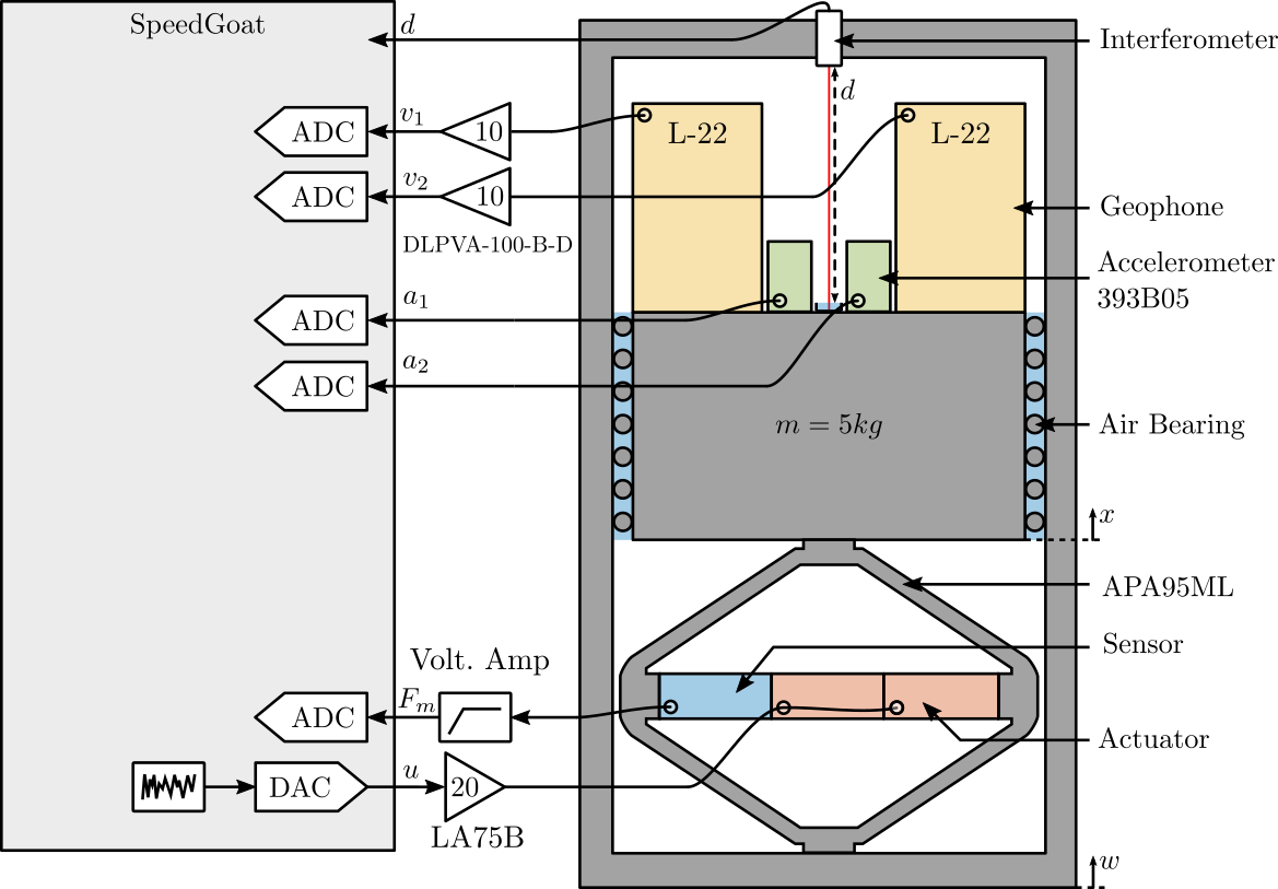
Figure 1: Schematic of the test-bench

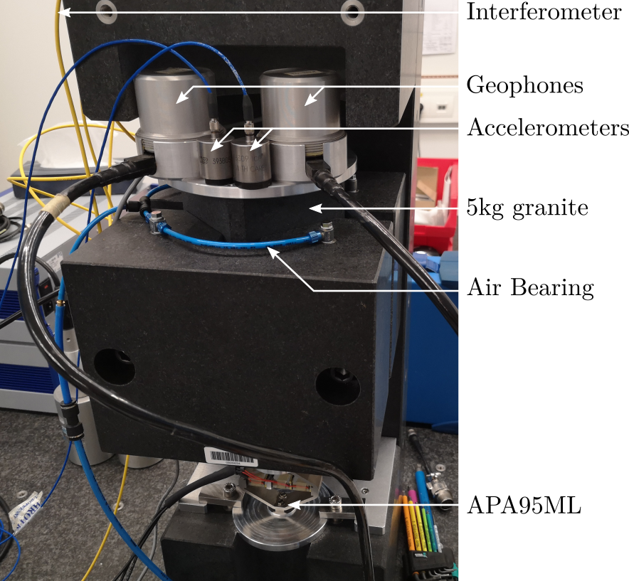
Figure 2: Picture of the test-bench

Two inertial sensors are used:

An vertical accelerometer PCB 393B05 (doc)
A vertical geophone Mark Product L-22

Basic characteristics of both sensors are shown in Tables 1 and 2.

Table 1: Accelerometer (393B05) Specifications
Specification	Value
Sensitivity	1.02 [V/(m/s2)]
Resonant Frequency	> 2.5 [kHz]
Resolution (1 to 10kHz)	0.00004 [m/s2 rms]

Table 2: Geophone (L22) Specifications
Specification	Value
Sensitivity	To be measured [V/(m/s)]
Resonant Frequency	2 [Hz]

The ADC used are the IO131 Speedgoat module (link) with a 16bit resolution over +/- 10V.

The geophone signals are amplified using a DLPVA-100-B-D voltage amplified from Femto (doc). The force sensor signal is amplified using a Low Noise Voltage Preamplifier from Ametek (doc).

The excitation signal is amplified by a linear amplified from Cedrat (LA75B) with a gain equals to 20 (doc).

Geophone electronics:

gain: 10 (20dB)
low pass filter: 1.5Hz
hifh pass filter: 100kHz (2nd order)

Force Sensor electronics:

gain: 10 (20dB)
low pass filter: 1st order at 3Hz
high pass filter: 1st order at 30kHz

2 First identification of the system

In this section, a first identification of each elements of the system is performed. This include the dynamics from the actuator to the force sensor, interferometer and inertial sensors.

Each of the dynamics is compared with the dynamics identified form a Simscape model.

2.1 Load Data

The data is loaded in the Matlab workspace.

Copy
  id_ol = load('identification_noise_bis.mat', 'd', 'acc_1', 'acc_2', 'geo_1', 'geo_2', 'f_meas', 'u', 't');

Then, any offset is removed.

Copy  id_ol.d      = detrend(id_ol.d, 0);
  id_ol.acc_1  = detrend(id_ol.acc_1, 0);
  id_ol.acc_2  = detrend(id_ol.acc_2, 0);
  id_ol.geo_1  = detrend(id_ol.geo_1, 0);
  id_ol.geo_2  = detrend(id_ol.geo_2, 0);
  id_ol.f_meas = detrend(id_ol.f_meas, 0);
  id_ol.u      = detrend(id_ol.u, 0);

2.2 Excitation Signal

The generated voltage used to excite the system is a white noise and can be seen in Figure 3.

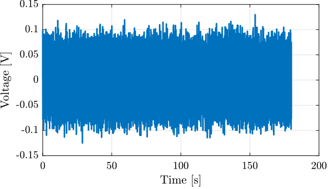
Figure 3: Voltage excitation signal

2.3 Identified Plant

The transfer function from the excitation voltage to the mass displacement and to the force sensor stack voltage are identified using the tfestimate command.

Copy
  Ts = id_ol.t(2) - id_ol.t(1);
  win = hann(ceil(10/Ts));

Copy
  [tf_fmeas_est, f] = tfestimate(id_ol.u, id_ol.f_meas, win, [], [], 1/Ts); % [V/V]
  [tf_G_ol_est,  ~] = tfestimate(id_ol.u, id_ol.d, win, [], [], 1/Ts); % [m/V]

The bode plots of the obtained dynamics are shown in Figures 4 and 5.

Figure 4: Bode plot of the dynamics from excitation voltage to measured force sensor stack voltage

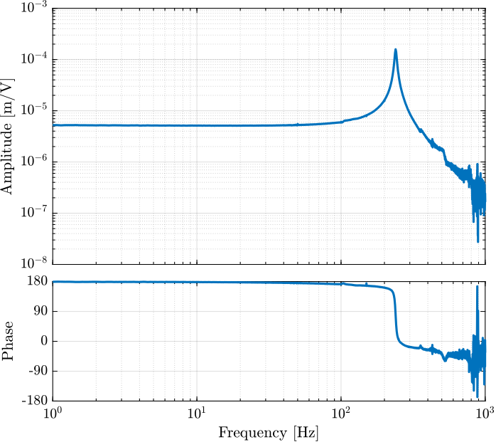
Figure 5: Bode plot of the dynamics from excitation voltage to displacement of the mass as measured by the interferometer

2.4 Simscape Model - Comparison

A simscape model representing the test-bench has been developed. The same transfer functions as the one identified using the test-bench can be obtained thanks to the simscape model.

They are compared in Figure 6 and 7. It is shown that there is a good agreement between the model and the experiment.

Copy
  load('piezo_amplified_3d.mat', 'int_xyz', 'int_i', 'n_xyz', 'n_i', 'nodes', 'M', 'K');

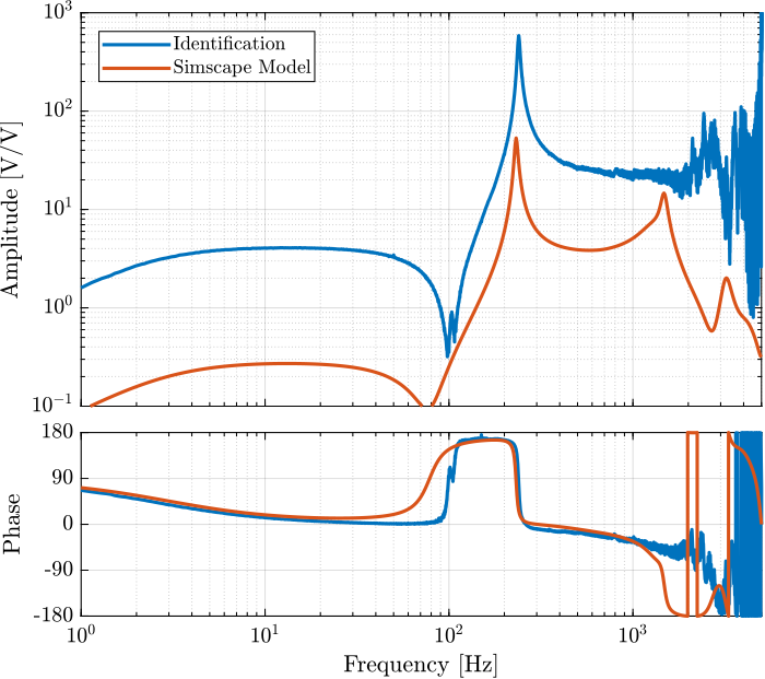
Figure 6: Comparison of the dynamics from excitation voltage to measured force sensor stack voltage - Identified dynamics and Simscape Model

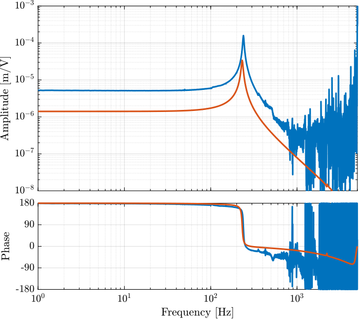
Figure 7: Comparison of the dynamics from excitation voltage to measured mass displacement - Identified dynamics and Simscape Model

2.5 Integral Force Feedback

The force sensor stack can be used to damp the system. This makes the system easier to excite properly without too much amplification near resonances.

This is done thanks to the integral force feedback control architecture.

The force sensor stack signal is integrated (or rather low pass filtered) and fed back to the force sensor stacks.

The low pass filter used as the controller is defined below:

Copy
  Kiff = 102/(s + 2*pi*2);

The integral force feedback control strategy is applied to the simscape model as well as to the real test bench.

The damped system is then identified again using a noise excitation.

The data is loaded into Matlab and any offset is removed.

Copy
  id_cl = load('identification_noise_iff_bis.mat', 'd', 'acc_1', 'acc_2', 'geo_1', 'geo_2', 'f_meas', 'u', 't');

  id_cl.d      = detrend(id_cl.d, 0);
  id_cl.acc_1  = detrend(id_cl.acc_1, 0);
  id_cl.acc_2  = detrend(id_cl.acc_2, 0);
  id_cl.geo_1  = detrend(id_cl.geo_1, 0);
  id_cl.geo_2  = detrend(id_cl.geo_2, 0);
  id_cl.f_meas = detrend(id_cl.f_meas, 0);
  id_cl.u      = detrend(id_cl.u, 0);

The transfer functions are estimated using tfestimate.

Copy
  [tf_G_cl_est, ~] = tfestimate(id_cl.u, id_cl.d, win, [], [], 1/Ts);
  [co_G_cl_est, ~] = mscohere(  id_cl.u, id_cl.d, win, [], [], 1/Ts);

The dynamics from driving voltage to the measured displacement are compared both in the open-loop and IFF case, and for the test-bench experimental identification and for the Simscape model in Figure 8. This shows that the Integral Force Feedback architecture effectively damps the first resonance of the system.

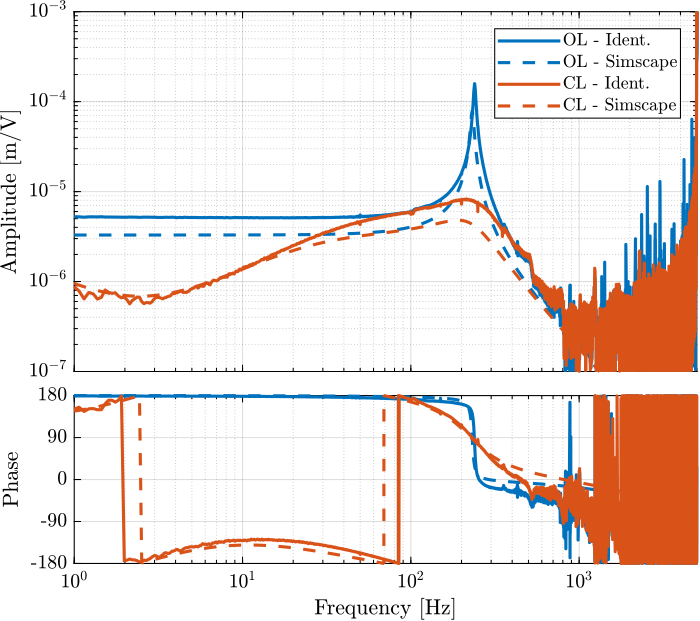
Figure 8: Comparison of the open-loop and closed-loop (IFF) dynamics for both the real identification and the Simscape one

2.6 Inertial Sensors

In order to estimate the dynamics of the inertial sensor (the transfer function from the “absolute” displacement to the measured voltage), the following experiment can be performed:

The mass is excited such that is relative displacement as measured by the interferometer is much larger that the ground “absolute” motion.
The transfer function from the measured displacement by the interferometer to the measured voltage generated by the inertial sensors can be estimated.

The first point is quite important in order to have a good coherence between the interferometer measurement and the inertial sensor measurement.

Here, a first identification is performed were the excitation signal is a white noise.

As usual, the data is loaded and any offset is removed.

Copy
  id = load('identification_noise_opt_iff.mat', 'd', 'acc_1', 'acc_2', 'geo_1', 'geo_2', 'f_meas', 'u', 't');

  id.d = detrend(id.d, 0);
  id.acc_1 = detrend(id.acc_1, 0);
  id.acc_2 = detrend(id.acc_2, 0);
  id.geo_1 = detrend(id.geo_1, 0);
  id.geo_2 = detrend(id.geo_2, 0);
  id.f_meas = detrend(id.f_meas, 0);

Then the transfer functions from the measured displacement by the interferometer to the generated voltage of the inertial sensors are computed..

Copy
  Ts = id.t(2) - id.t(1);
  win = hann(ceil(10/Ts));

Copy
  [tf_acc1_est, f] = tfestimate(id.d, id.acc_1, win, [], [], 1/Ts);
  [co_acc1_est, ~] = mscohere(  id.d, id.acc_1, win, [], [], 1/Ts);
  [tf_acc2_est, ~] = tfestimate(id.d, id.acc_2, win, [], [], 1/Ts);
  [co_acc2_est, ~] = mscohere(  id.d, id.acc_2, win, [], [], 1/Ts);

  [tf_geo1_est, ~] = tfestimate(id.d, id.geo_1, win, [], [], 1/Ts);
  [co_geo1_est, ~] = mscohere(  id.d, id.geo_1, win, [], [], 1/Ts);
  [tf_geo2_est, ~] = tfestimate(id.d, id.geo_2, win, [], [], 1/Ts);
  [co_geo2_est, ~] = mscohere(  id.d, id.geo_2, win, [], [], 1/Ts);

The same transfer functions are estimated using the Simscape model.

The obtained dynamics of the accelerometer are compared in Figure 9 while the one of the geophones are compared in Figure 10.

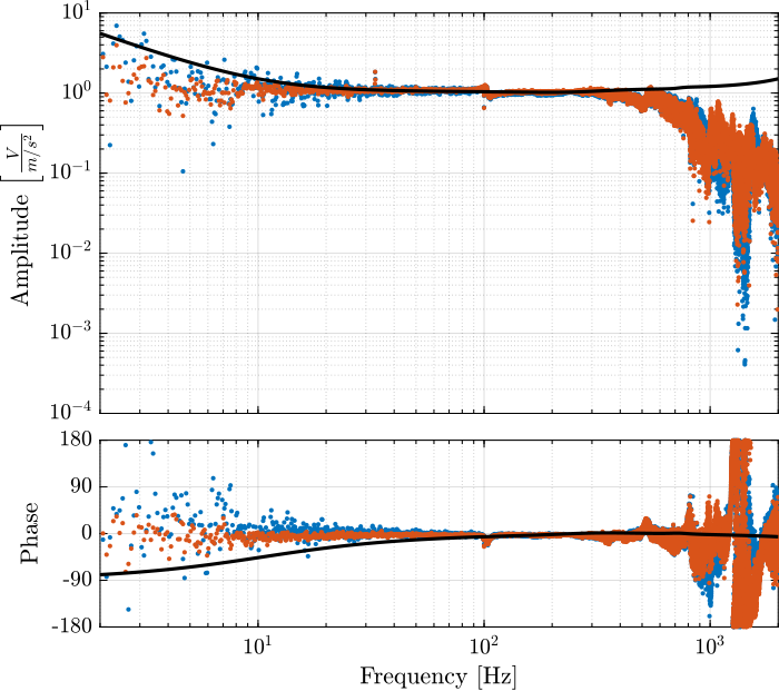
Figure 9: Comparison of the measured accelerometer dynamics

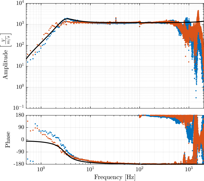
Figure 10: Comparison of the measured geophone dynamics

3 Optimal IFF Development

In this section, a proper identification of the transfer function from the force actuator to the force sensor is performed. Then, an optimal IFF controller is developed and applied experimentally.

The damped system is identified to verified the effectiveness of the added method.

3.1 Load Data

The experimental data is loaded and any offset is removed.

Copy
  id_ol = load('identification_noise_bis.mat', 'd', 'acc_1', 'acc_2', 'geo_1', 'geo_2', 'f_meas', 'u', 't');

Copy  id_ol.d = detrend(id_ol.d, 0);
  id_ol.acc_1 = detrend(id_ol.acc_1, 0);
  id_ol.acc_2 = detrend(id_ol.acc_2, 0);
  id_ol.geo_1 = detrend(id_ol.geo_1, 0);
  id_ol.geo_2 = detrend(id_ol.geo_2, 0);
  id_ol.f_meas = detrend(id_ol.f_meas, 0);
  id_ol.u = detrend(id_ol.u, 0);

3.2 Experimental Data

The transfer function from force actuator to force sensors is estimated.

The coherence shown in Figure 11 shows that the excitation signal is good enough.

Copy
  Ts = id_ol.t(2) - id_ol.t(1);
  win = hann(ceil(10/Ts));

Copy
  [tf_fmeas_est, f] = tfestimate(id_ol.u, id_ol.f_meas, win, [], [], 1/Ts); % [V/m]
  [co_fmeas_est, ~] = mscohere(  id_ol.u, id_ol.f_meas, win, [], [], 1/Ts);

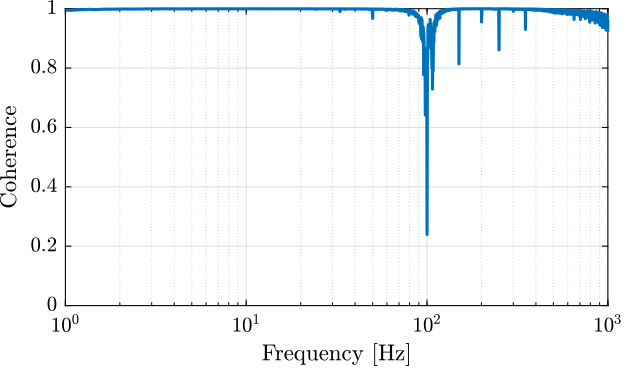
Figure 11: Coherence for the identification of the IFF plant

The obtained dynamics is shown in Figure 12.

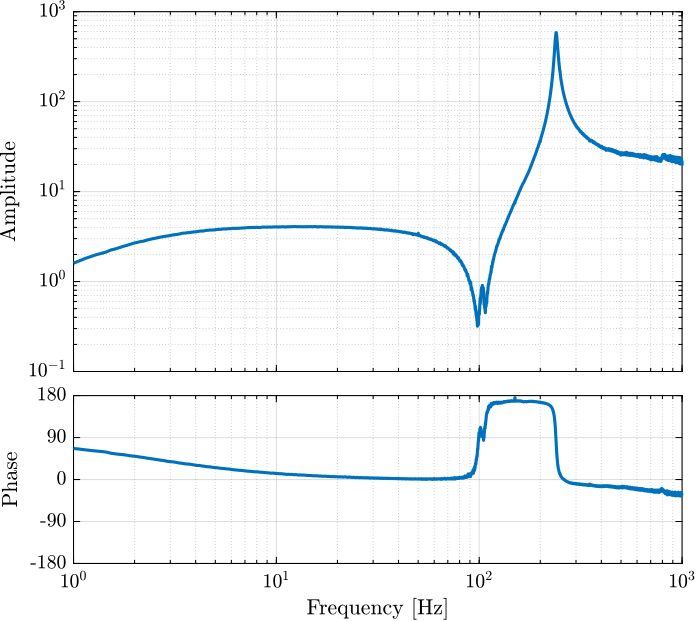
Figure 12: Bode plot of the identified IFF plant

3.3 Model of the IFF Plant

In order to plot the root locus for the IFF control strategy, a model of the identified plant is developed.

It consists of several poles and zeros are shown below.

Copy
  wz = 2*pi*102;
  xi_z = 0.01;
  wp = 2*pi*239.4;
  xi_p = 0.015;

  Giff = 2.2*(s^2 + 2*xi_z*s*wz + wz^2)/(s^2 + 2*xi_p*s*wp + wp^2) * ... % Dynamics
         10*(s/3/pi/(1 + s/3/pi)) * ... % Low pass filter and gain of the voltage amplifier
         exp(-Ts*s); % Time delay induced by ADC/DAC

The comparison of the identified dynamics and the developed model is done in Figure 13.

Figure 13: IFF Plant + Model

3.4 Root Locus and optimal Controller

Now, the root locus for the Integral Force Feedback strategy is computed and shown in Figure 14.

Note that the controller used is not a pure integrator but rather a first order low pass filter with a cut-off frequency set at 2Hz.

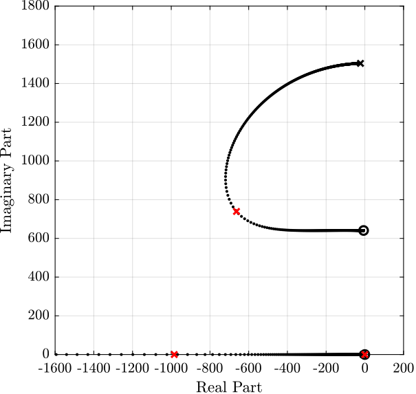
Figure 14: Root Locus for the IFF control

The controller that yield maximum damping (shown by the red cross in Figure 14) is:

Copy
  Kiff_opt = 102/(s + 2*pi*2);

3.5 Verification of the achievable damping

A new identification is performed with the IFF control strategy applied to the system.

Data is loaded and offset removed.

Copy
  id_cl = load('identification_noise_iff_bis.mat', 'd', 'acc_1', 'acc_2', 'geo_1', 'geo_2', 'f_meas', 'u', 't');

Copy  id_cl.d      = detrend(id_cl.d, 0);
  id_cl.acc_1  = detrend(id_cl.acc_1, 0);
  id_cl.acc_2  = detrend(id_cl.acc_2, 0);
  id_cl.geo_1  = detrend(id_cl.geo_1, 0);
  id_cl.geo_2  = detrend(id_cl.geo_2, 0);
  id_cl.f_meas = detrend(id_cl.f_meas, 0);
  id_cl.u      = detrend(id_cl.u, 0);

The open-loop and closed-loop dynamics are estimated.

Copy
  [tf_G_ol_est, f] = tfestimate(id_ol.u, id_ol.d, win, [], [], 1/Ts);
  [co_G_ol_est, ~] = mscohere(  id_ol.u, id_ol.d, win, [], [], 1/Ts);
  [tf_G_cl_est, ~] = tfestimate(id_cl.u, id_cl.d, win, [], [], 1/Ts);
  [co_G_cl_est, ~] = mscohere(  id_cl.u, id_cl.d, win, [], [], 1/Ts);

The obtained coherence is shown in Figure 15 and the dynamics in Figure 16.

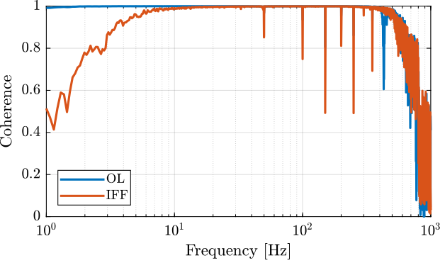
Figure 15: Coherence for the transfer function from F to d, with and without IFF

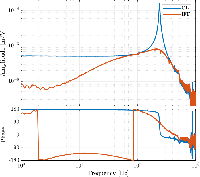
Figure 16: Coherence for the transfer function from F to d, with and without IFF

4 Generate the excitation signal

In order to properly estimate the dynamics of the inertial sensor, the excitation signal must be properly chosen.

The requirements on the excitation signal is:

General much larger motion that the measured motion during the huddle test
Don’t damage the actuator

To determine the perfect voltage signal to be generated, we need two things:

the transfer function from voltage to mass displacement
the PSD of the measured motion by the inertial sensors
not saturate the sensor signals
provide enough signal/noise ratio (good coherence) in the frequency band of interest (~0.5Hz to 3kHz)

4.1 Transfer function from excitation signal to displacement

Let’s first estimate the transfer function from the excitation signal in [V] to the generated displacement in [m] as measured by the inteferometer.

Copy
  id_cl = load('identification_noise_iff_bis.mat', 'd', 'acc_1', 'acc_2', 'geo_1', 'geo_2', 'f_meas', 'u', 't');

Copy
  Ts = id_cl.t(2) - id_cl.t(1);
  win = hann(ceil(10/Ts));

Copy
  [tf_G_cl_est, f] = tfestimate(id_cl.u, id_cl.d, win, [], [], 1/Ts);
  [co_G_cl_est, ~] = mscohere(  id_cl.u, id_cl.d, win, [], [], 1/Ts);

Approximate transfer function from voltage output to generated displacement when IFF is used, in [m/V].

Copy
  G_d_est = -5e-6*(2*pi*230)^2/(s^2 + 2*0.3*2*pi*240*s + (2*pi*240)^2);

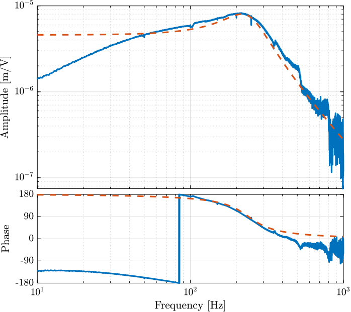
Figure 17: Estimation of the transfer function from the excitation signal to the generated displacement

4.2 Motion measured during Huddle test

We now compute the PSD of the measured motion by the inertial sensors during the huddle test.

Copy
  ht = load('huddle_test.mat', 'd', 'acc_1', 'acc_2', 'geo_1', 'geo_2', 'f_meas', 'u', 't');
  ht.d = detrend(ht.d, 0);
  ht.acc_1 = detrend(ht.acc_1, 0);
  ht.acc_2 = detrend(ht.acc_2, 0);
  ht.geo_1 = detrend(ht.geo_1, 0);
  ht.geo_2 = detrend(ht.geo_2, 0);

Copy
  [p_d, f] = pwelch(ht.d, win, [], [], 1/Ts);
  [p_acc1, ~] = pwelch(ht.acc_1, win, [], [], 1/Ts);
  [p_acc2, ~] = pwelch(ht.acc_2, win, [], [], 1/Ts);
  [p_geo1, ~] = pwelch(ht.geo_1, win, [], [], 1/Ts);
  [p_geo2, ~] = pwelch(ht.geo_2, win, [], [], 1/Ts);

Using an estimated model of the sensor dynamics from the documentation of the sensors, we can compute the ASD of the motion in $m / \sqrt{H z}$ measured by the sensors.

Copy
  G_acc = 1/(1 + s/2/pi/2500); % [V/(m/s2)]
  G_geo = -120*s^2/(s^2 + 2*0.7*2*pi*2*s + (2*pi*2)^2); % [V/(m/s)]

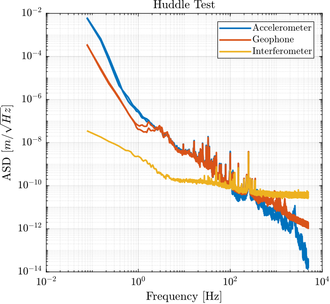
Figure 18: ASD of the motion measured by the sensors

From the ASD of the motion measured by the sensors, we can create an excitation signal that will generate much motion motion that the motion under no excitation.

We create G_exc that corresponds to the wanted generated motion.

Copy
  G_exc = 0.2e-6/(1 + s/2/pi/2)/(1 + s/2/pi/50);

And we create a time domain signal y_d that have the spectral density described by G_exc.

Copy
  Fs = 1/Ts;
  t = 0:Ts:180; % Time Vector [s]
  u = sqrt(Fs/2)*randn(length(t), 1); % Signal with an ASD equal to one

  y_d = lsim(G_exc, u, t);

Copy
  [pxx, ~] = pwelch(y_d, win, 0, [], Fs);

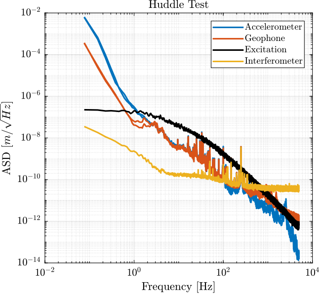
Figure 19: Comparison of the ASD of the motion during Huddle and the wanted generated motion

We can now generate the voltage signal that will generate the wanted motion.

Copy
  y_v = lsim(G_exc * ... % from unit PSD to shaped PSD
             (1 + s/2/pi/50) * ... % Inverse of pre-filter included in the Simulink file
             1/G_d_est * ... % Wanted displacement => required voltage
             1/(1 + s/2/pi/5e3), ... %  Add some high frequency filtering
             u, t);

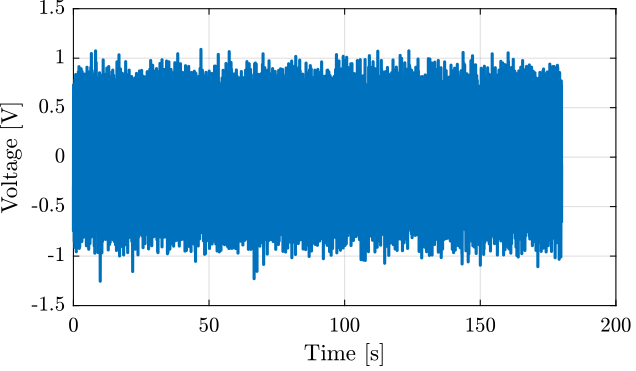
Figure 20: Generated excitation signal

5 Identification of the Inertial Sensors Dynamics

Using the excitation signal generated in Section 4, the dynamics of the inertial sensors are identified.

5.1 Load Data

Both the measurement data during the identification test and during an “huddle test” are loaded.

Copy
  id = load('identification_noise_opt_iff.mat', 'd', 'acc_1', 'acc_2', 'geo_1', 'geo_2', 'f_meas', 'u', 't');
  ht = load('huddle_test.mat', 'd', 'acc_1', 'acc_2', 'geo_1', 'geo_2', 'f_meas', 'u', 't');

Copy  ht.d = detrend(ht.d, 0);
  ht.acc_1 = detrend(ht.acc_1, 0);
  ht.acc_2 = detrend(ht.acc_2, 0);
  ht.geo_1 = detrend(ht.geo_1, 0);
  ht.geo_2 = detrend(ht.geo_2, 0);
  ht.f_meas = detrend(ht.f_meas, 0);

Copy  id.d = detrend(id.d, 0);
  id.acc_1 = detrend(id.acc_1, 0);
  id.acc_2 = detrend(id.acc_2, 0);
  id.geo_1 = detrend(id.geo_1, 0);
  id.geo_2 = detrend(id.geo_2, 0);
  id.f_meas = detrend(id.f_meas, 0);

5.2 Compare PSD during Huddle and and during identification

The Power Spectral Density of the measured motion during the huddle test and during the identification test are compared in Figures 21 and 22.

Copy
  Ts = ht.t(2) - ht.t(1);
  win = hann(ceil(10/Ts));

Copy
  [p_id_d, f] = pwelch(id.d, win, [], [], 1/Ts);
  [p_id_acc1, ~] = pwelch(id.acc_1, win, [], [], 1/Ts);
  [p_id_acc2, ~] = pwelch(id.acc_2, win, [], [], 1/Ts);
  [p_id_geo1, ~] = pwelch(id.geo_1, win, [], [], 1/Ts);
  [p_id_geo2, ~] = pwelch(id.geo_2, win, [], [], 1/Ts);

Copy
  [p_ht_d, ~] = pwelch(ht.d, win, [], [], 1/Ts);
  [p_ht_acc1, ~] = pwelch(ht.acc_1, win, [], [], 1/Ts);
  [p_ht_acc2, ~] = pwelch(ht.acc_2, win, [], [], 1/Ts);
  [p_ht_geo1, ~] = pwelch(ht.geo_1, win, [], [], 1/Ts);
  [p_ht_geo2, ~] = pwelch(ht.geo_2, win, [], [], 1/Ts);
  [p_ht_fmeas, ~] = pwelch(ht.f_meas, win, [], [], 1/Ts);

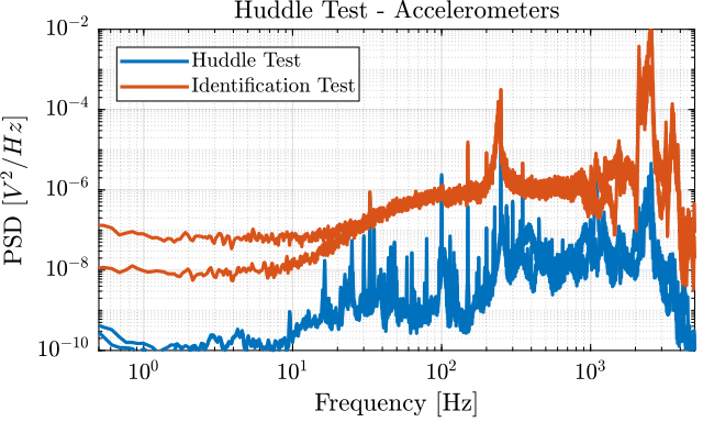
Figure 21: Comparison of the PSD of the measured motion during the Huddle test and during the identification

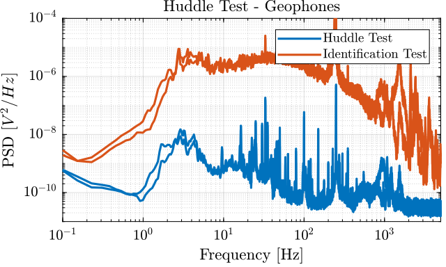
Figure 22: Comparison of the PSD of the measured motion during the Huddle test and during the identification

5.3 Compute transfer functions

The transfer functions from the motion as measured by the interferometer (and that should represent the absolute motion of the mass) to the inertial sensors are estimated:

Copy
  [tf_acc1_est, f] = tfestimate(id.d, id.acc_1, win, [], [], 1/Ts);
  [co_acc1_est, ~] = mscohere(  id.d, id.acc_1, win, [], [], 1/Ts);
  [tf_acc2_est, ~] = tfestimate(id.d, id.acc_2, win, [], [], 1/Ts);
  [co_acc2_est, ~] = mscohere(  id.d, id.acc_2, win, [], [], 1/Ts);

  [tf_geo1_est, ~] = tfestimate(id.d, id.geo_1, win, [], [], 1/Ts);
  [co_geo1_est, ~] = mscohere(  id.d, id.geo_1, win, [], [], 1/Ts);
  [tf_geo2_est, ~] = tfestimate(id.d, id.geo_2, win, [], [], 1/Ts);
  [co_geo2_est, ~] = mscohere(  id.d, id.geo_2, win, [], [], 1/Ts);

The obtained coherence are shown in Figure 23.

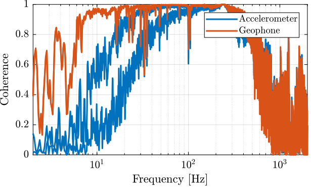
Figure 23: Coherence for the estimation of the sensor dynamics

We also make a simplified model of the inertial sensors to be compared with the identified dynamics.

Copy
  G_acc = 1/(1 + s/2/pi/2500); % [V/(m/s2)]
  G_geo = -1200*s^2/(s^2 + 2*0.7*2*pi*2*s + (2*pi*2)^2); % [[V/(m/s)]

The model and identified dynamics show good agreement (Figures 24 and 25.)

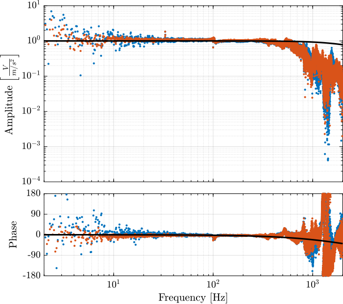
Figure 24: Identified dynamics of the accelerometers

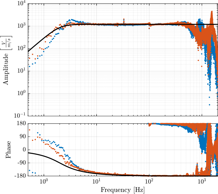
Figure 25: Identified dynamics of the geophones

6 Inertial Sensor Noise and the $H_{2}$ Synthesis of complementary filters

In this section, the noise of the inertial sensors (geophones and accelerometers) is estimated.

6.1 Load Data

As before, the identification data is loaded and any offset if removed.

Copy
  id = load('identification_noise_opt_iff.mat', 'd', 'acc_1', 'acc_2', 'geo_1', 'geo_2', 'f_meas', 'u', 't');

Copy  id.d = detrend(id.d, 0);
  id.acc_1 = detrend(id.acc_1, 0);
  id.acc_2 = detrend(id.acc_2, 0);
  id.geo_1 = detrend(id.geo_1, 0);
  id.geo_2 = detrend(id.geo_2, 0);
  id.f_meas = detrend(id.f_meas, 0);

6.2 ASD of the Measured displacement

The Power Spectral Density of the displacement as measured by the interferometer and the inertial sensors is computed.

Copy
  Ts = id.t(2) - id.t(1);
  win = hann(ceil(10/Ts));

Copy
  [p_id_d,     f] = pwelch(id.d,      win, [], [], 1/Ts);
  [p_id_acc1,  ~] = pwelch(id.acc_1,  win, [], [], 1/Ts);
  [p_id_acc2,  ~] = pwelch(id.acc_2,  win, [], [], 1/Ts);
  [p_id_geo1,  ~] = pwelch(id.geo_1,  win, [], [], 1/Ts);
  [p_id_geo2,  ~] = pwelch(id.geo_2,  win, [], [], 1/Ts);

Let’s use a model of the accelerometer and geophone to compute the motion from the measured voltage.

Copy
  G_acc = 1/(1 + s/2/pi/2500); % [V/(m/s2)]
  G_geo = -1200*s^2/(s^2 + 2*0.7*2*pi*2*s + (2*pi*2)^2); % [[V/(m/s)]

The obtained ASD in $m / \sqrt{H z}$ is shown in Figure 26.

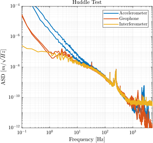
Figure 26: ASD of the measured displacement as measured by all the sensors

6.3 ASD of the Sensor Noise

The noise of a sensor can be estimated using two identical sensors by computing:

the Power Spectral Density of the measured motion by the two sensors
the Cross Spectral Density between the two sensors (coherence)

This technique to estimate the sensor noise is described in (Barzilai, VanZandt, and Kenny 1998).

The Power Spectral Density of the sensor noise can be estimated using the following equation:

\begin{matrix} (1) & | S_{n} (ω) | = | S_{x_{1}} (ω) | (1 - γ_{x_{1} x_{2}} (ω)) \end{matrix}

with $S_{x_{1}}$ the PSD of one of the sensor and $γ_{x_{1} x_{2}}$ the coherence between the two sensors.

The coherence between the two accelerometers and between the two geophones is computed.

Copy
  [coh_acc, ~] = mscohere(id.acc_1, id.acc_2, win, [], [], 1/Ts);
  [coh_geo, ~] = mscohere(id.geo_1, id.geo_2, win, [], [], 1/Ts);

Finally, the Power Spectral Density of the sensors is computed and converted in $[m^{2} / H z]$ .

Copy
  pN_acc = p_id_acc1.*(1 - coh_acc) .* ... % [V^2/Hz]
           1./abs(squeeze(freqresp(G_acc*s^2, f, 'Hz'))).^2; % [(m/V)^2]
  pN_geo = p_id_geo1.*(1 - coh_geo) .* ... % [V^2/Hz]
           1./abs(squeeze(freqresp(G_geo*s, f, 'Hz'))).^2; % [(m/V)^2]

The ASD of obtained noises are compared with the ASD of the measured signals in Figure 27.

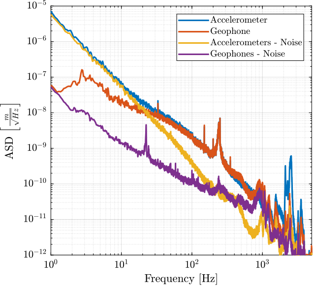
Figure 27: Comparison of the computed ASD of the noise of the two inertial sensors

6.4 Noise Model

Transfer functions are adjusted in order to fit the ASD of the sensor noises (expressed in $[m / s / \sqrt{H z}]$ for more easy fitting).

These transfer functions are defined below and compared with the measured ASD in Figure 28.

Copy
  N_acc = 1*(s/(2*pi*2000) + 1)^2/(s + 0.1*2*pi)/(s + 1e3*2*pi); % [m/sqrt(Hz)]
  N_geo = 4e-4*(s/(2*pi*200) + 1)/(s + 1e3*2*pi); % [m/sqrt(Hz)]

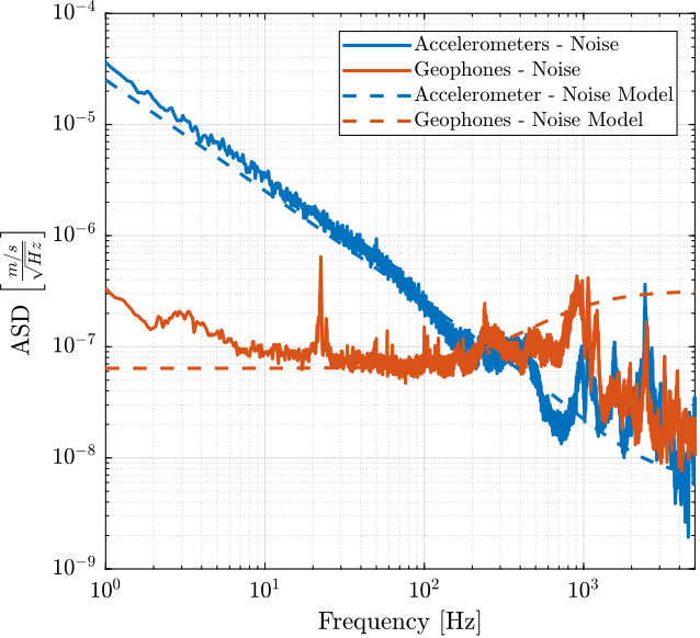
Figure 28: ASD of the velocity noise measured by the sensors and the noise models

6.5 $H_{2}$ Synthesis of the Complementary Filters

We now wish to synthesize two complementary filters to merge the geophone and the accelerometer signal in such a way that the fused signal has the lowest possible RMS noise.

To do so, we use the $H_{2}$ synthesis where the transfer functions representing the noise density of both sensors are used as weights.

The generalized plant used for the synthesis is defined below.

Copy  P = [0      N_acc  1;
       N_geo -N_acc  0];

And the $H_{2}$ synthesis is done using the h2syn command.

Copy
  [H_geo, ~, gamma] = h2syn(P, 1, 1);
  H_acc = 1 - H_geo;

The obtained complementary filters are shown in Figure 29.

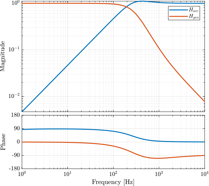
Figure 29: Obtained Complementary Filters

6.6 Results

Finally, the signals of both sensors are merged using the complementary filters and the super sensor noise is estimated and compared with the individual sensor noises in Figure 30.

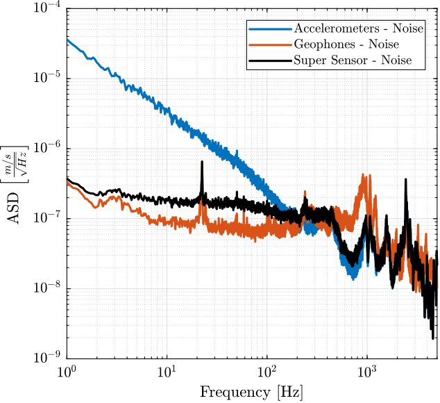
Figure 30: ASD of the super sensor noise (velocity)

Finally, the Cumulative Power Spectrum is computed and compared in Figure 31.

Copy
  [~, i_1Hz] = min(abs(f - 1));

Copy
  CPS_acc = 1/pi*flip(-cumtrapz(2*pi*flip(f), flip((pN_acc.*(2*pi*f)).^2)));
  CPS_geo = 1/pi*flip(-cumtrapz(2*pi*flip(f), flip((pN_geo.*(2*pi*f)).^2)));
  CPS_SS  = 1/pi*flip(-cumtrapz(2*pi*flip(f), flip((pN_acc.*(2*pi*f)).^2.*abs(squeeze(freqresp(H_acc, f, 'Hz'))).^2 + (pN_geo.*(2*pi*f)).^2.*abs(squeeze(freqresp(H_geo, f, 'Hz'))).^2)));

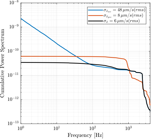
Figure 31: Cumulative Power Spectrum of the Sensor Noise (velocity)

7 Inertial Sensor Dynamics Uncertainty and the $H_{\infty}$ Synthesis of complementary filters

When merging two sensors, it is important to be sure that we correctly know the sensor dynamics near the merging frequency. Thus, identifying the uncertainty on the sensor dynamics is quite important to perform a robust merging.

7.1 Load Data

Data is loaded and offset is removed.

Copy
  id = load('identification_noise_opt_iff.mat', 'd', 'acc_1', 'acc_2', 'geo_1', 'geo_2', 'f_meas', 'u', 't');

Copy  id.d = detrend(id.d, 0);
  id.acc_1 = detrend(id.acc_1, 0);
  id.acc_2 = detrend(id.acc_2, 0);
  id.geo_1 = detrend(id.geo_1, 0);
  id.geo_2 = detrend(id.geo_2, 0);
  id.f_meas = detrend(id.f_meas, 0);

7.2 Compute the dynamics of both sensors

The dynamics of inertial sensors are estimated (in $[V / m]$ ).

Copy
  Ts = id.t(2) - id.t(1);
  win = hann(ceil(10/Ts));

Copy
  [tf_acc1_est, f] = tfestimate(id.d, id.acc_1, win, [], [], 1/Ts);
  [co_acc1_est, ~] = mscohere(  id.d, id.acc_1, win, [], [], 1/Ts);
  [tf_acc2_est, ~] = tfestimate(id.d, id.acc_2, win, [], [], 1/Ts);
  [co_acc2_est, ~] = mscohere(  id.d, id.acc_2, win, [], [], 1/Ts);

  [tf_geo1_est, ~] = tfestimate(id.d, id.geo_1, win, [], [], 1/Ts);
  [co_geo1_est, ~] = mscohere(  id.d, id.geo_1, win, [], [], 1/Ts);
  [tf_geo2_est, ~] = tfestimate(id.d, id.geo_2, win, [], [], 1/Ts);
  [co_geo2_est, ~] = mscohere(  id.d, id.geo_2, win, [], [], 1/Ts);

The (nominal) models of the inertial sensors from the absolute displacement to the generated voltage are defined below:

Copy
  G_acc = 1/(1 + s/2/pi/2000)
  G_geo = -1200*s^2/(s^2 + 2*0.7*2*pi*2*s + (2*pi*2)^2);

These models are very simplistic models, and we then take into account the un-modelled dynamics with dynamical uncertainty.

7.3 Dynamics uncertainty estimation

Weights representing the dynamical uncertainty of the sensors are defined below.

Copy
  w_acc = createWeight('n', 2, 'G0', 10,  'G1', 0.2,    'Gc', 1,     'w0', 6*2*pi) * ...
          createWeight('n', 2, 'G0', 1,   'G1', 5/0.2,  'Gc', 1/0.2, 'w0', 1300*2*pi);

  w_geo = createWeight('n', 2, 'G0', 0.6, 'G1', 0.2,    'Gc', 0.3,   'w0', 3*2*pi) * ...
          createWeight('n', 2, 'G0', 1,   'G1', 10/0.2, 'Gc', 1/0.2, 'w0', 800*2*pi);

The measured dynamics are compared with the modelled one as well as the modelled uncertainty in Figure 32 for the accelerometers and in Figure 33 for the geophones.

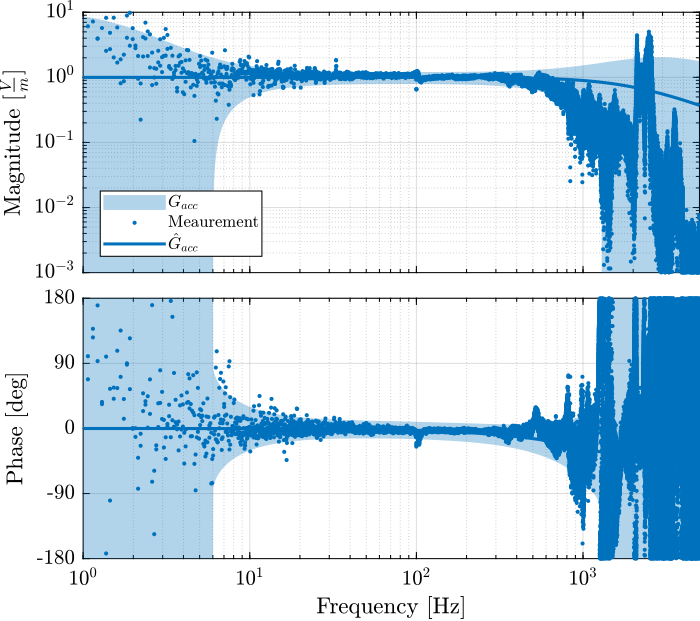
Figure 32: Modeled dynamical uncertainty and meaured dynamics of the accelerometers

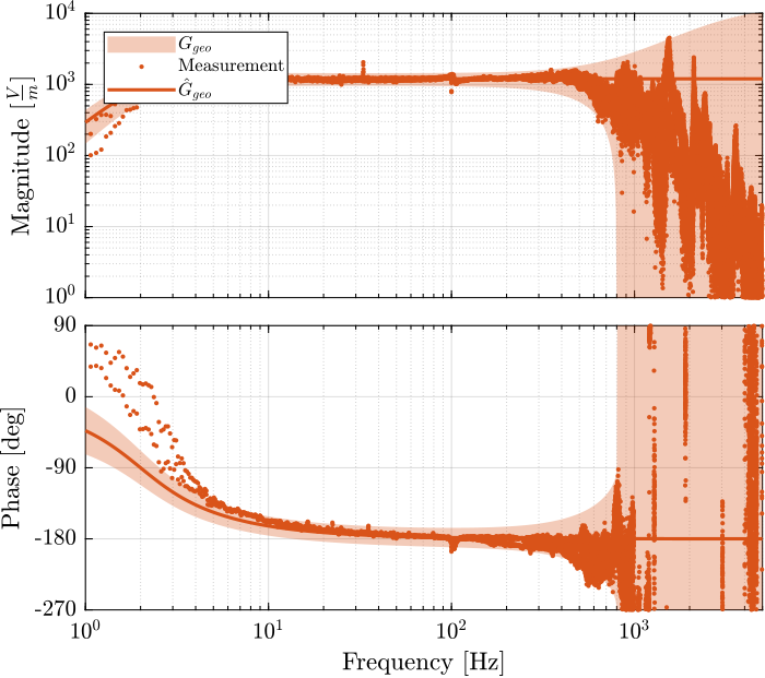
Figure 33: Modeled dynamical uncertainty and meaured dynamics of the geophones

7.4 $H_{\infty}$ Synthesis of Complementary Filters

A last weight is now defined that represents the maximum dynamical uncertainty that is allowed for the super sensor.

Copy
  wu = inv(createWeight('n', 2, 'G0', 0.7, 'G1', 0.3,   'Gc', 0.4,   'w0', 3*2*pi) * ...
           createWeight('n', 2, 'G0', 1,   'G1', 6/0.3, 'Gc', 1/0.3, 'w0', 1200*2*pi));

This dynamical uncertainty is compared with the two sensor uncertainties in Figure 34.

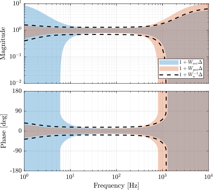
Figure 34: Individual sensor uncertainty (normalized by their dynamics) and the wanted maximum super sensor noise uncertainty

The generalized plant used for the synthesis is defined:

Copy
  P = [wu*w_acc -wu*w_acc;
       0         wu*w_geo;
       1         0];

And the $H_{\infty}$ synthesis using the hinfsyn command is performed.

Copy
  [H_geo, ~, gamma, ~] = hinfsyn(P, 1, 1,'TOLGAM', 0.001, 'METHOD', 'ric', 'DISPLAY', 'on');

  Test bounds:  0.8556 <=  gamma  <=  1.34

    gamma        X>=0        Y>=0       rho(XY)<1    p/f
  1.071e+00     0.0e+00     0.0e+00     0.000e+00     p
  9.571e-01     0.0e+00     0.0e+00     9.436e-16     p
  9.049e-01     0.0e+00     0.0e+00     1.084e-15     p
  8.799e-01     0.0e+00     0.0e+00     1.191e-16     p
  8.677e-01     0.0e+00     0.0e+00     6.905e-15     p
  8.616e-01     0.0e+00     0.0e+00     0.000e+00     p
  8.586e-01     1.1e-17     0.0e+00     6.917e-16     p
  8.571e-01     0.0e+00     0.0e+00     6.991e-17     p
  8.564e-01     0.0e+00     0.0e+00     1.492e-16     p

  Best performance (actual): 0.8563

The complementary filter is defined as follows:

Copy
  H_acc = 1 - H_geo;

The bode plot of the obtained complementary filters is shown in Figure

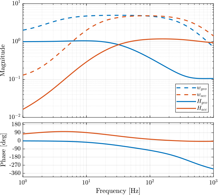
Figure 35: Bode plot of the obtained complementary filters using the $H_{\infty}$ synthesis

7.5 Obtained Super Sensor Dynamical Uncertainty

The obtained super sensor dynamical uncertainty is shown in Figure 36.

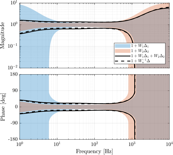
Figure 36: Obtained Super sensor dynamics uncertainty

8 Optimal and Robust sensor fusion using the $H_{2} / H_{\infty}$ synthesis

8.1 Noise and Dynamical uncertainty weights

Copy
  N_acc = (s/(2*pi*2000) + 1)^2/(s + 0.1*2*pi)/(s + 1e3*2*pi)/(1 + s/2/pi/1e3); % [m/sqrt(Hz)]
  N_geo = 4e-4*((s + 2*pi)/(2*pi*200) + 1)/(s + 1e3*2*pi)/(1 + s/2/pi/1e3); % [m/sqrt(Hz)]

Copy
  w_acc = createWeight('n', 2, 'G0', 10,  'G1', 0.2,    'Gc', 1,     'w0', 6*2*pi) * ...
          createWeight('n', 2, 'G0', 1,   'G1', 5/0.2,  'Gc', 1/0.2, 'w0', 1300*2*pi);

  w_geo = createWeight('n', 2, 'G0', 0.6, 'G1', 0.2,    'Gc', 0.3,   'w0', 3*2*pi) * ...
          createWeight('n', 2, 'G0', 1,   'G1', 10/0.2, 'Gc', 1/0.2, 'w0', 800*2*pi);

Copy
  wu = inv(createWeight('n', 2, 'G0', 0.7, 'G1', 0.3,   'Gc', 0.4,   'w0', 3*2*pi) * ...
           createWeight('n', 2, 'G0', 1,   'G1', 6/0.3, 'Gc', 1/0.3, 'w0', 1200*2*pi));

Copy
  P = [wu*w_acc -wu*w_acc;
       0         wu*w_geo;
       N_acc    -N_acc;
       0         N_geo;
       1         0];

And the mixed $H_{2} / H_{\infty}$ synthesis is performed.

Copy
  [H_geo, ~] = h2hinfsyn(ss(P), 1, 1, 2, [0, 1], 'HINFMAX', 1, 'H2MAX', Inf, 'DKMAX', 100, 'TOL', 1e-3, 'DISPLAY', 'on');

Copy
  H_acc = 1 - H_geo;

8.2 Obtained Super Sensor Noise

Copy  freqs = logspace(0, 4, 1000);
  PSD_Sgeo = abs(squeeze(freqresp(N_geo, freqs, 'Hz'))).^2;
  PSD_Sacc = abs(squeeze(freqresp(N_acc, freqs, 'Hz'))).^2;
  PSD_Hss  = abs(squeeze(freqresp(N_acc*H_acc, freqs, 'Hz'))).^2 + ...
             abs(squeeze(freqresp(N_geo*H_geo, freqs, 'Hz'))).^2;

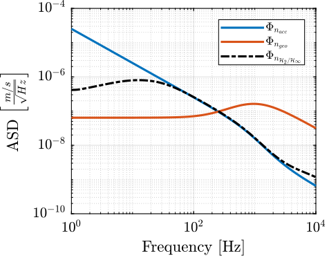
Figure 37: Power Spectral Density of the Super Sensor obtained with the mixed $H_{2} / H_{\infty}$ synthesis

8.3 Obtained Super Sensor Dynamical Uncertainty

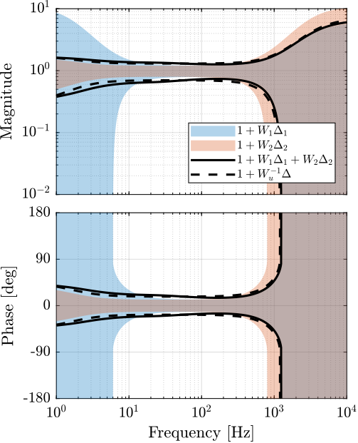
Figure 38: Super sensor dynamical uncertainty (solid curve) when using the mixed $H_{2} / H_{\infty}$ Synthesis

8.4 Experimental Super Sensor Dynamical Uncertainty

The super sensor dynamics is shown in Figure 39.

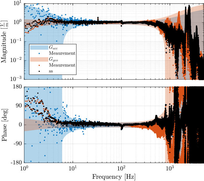
Figure 39: Inertial Sensor dynamics as well as the super sensor dynamics

8.5 Experimental Super Sensor Noise

The obtained super sensor noise is shown in Figure 40.

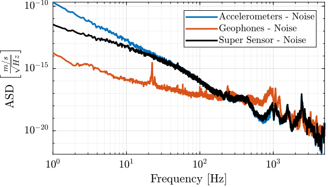
Figure 40: ASD of the super sensor obtained using the $H_{2} / H_{\infty}$ synthesis

9 Matlab Functions

9.1 `createWeight`

This Matlab function is accessible here.

Copy
    function [W] = createWeight(args)
    % createWeight -
    %
    % Syntax: [in_data] = createWeight(in_data)
    %
    % Inputs:
    %    - n  - Weight Order
    %    - G0 - Low frequency Gain
    %    - G1 - High frequency Gain
    %    - Gc - Gain of W at frequency w0
    %    - w0 - Frequency at which |W(j w0)| = Gc
    %
    % Outputs:
    %    - W - Generated Weight

        arguments
            args.n  (1,1) double {mustBeInteger, mustBePositive} = 1
            args.G0 (1,1) double {mustBeNumeric, mustBePositive} = 0.1
            args.G1 (1,1) double {mustBeNumeric, mustBePositive} = 10
            args.Gc (1,1) double {mustBeNumeric, mustBePositive} = 1
            args.w0 (1,1) double {mustBeNumeric, mustBePositive} = 1
        end

      mustBeBetween(args.G0, args.Gc, args.G1);

      s = tf('s');

      W = (((1/args.w0)*sqrt((1-(args.G0/args.Gc)^(2/args.n))/(1-(args.Gc/args.G1)^(2/args.n)))*s + (args.G0/args.Gc)^(1/args.n))/((1/args.G1)^(1/args.n)*(1/args.w0)*sqrt((1-(args.G0/args.Gc)^(2/args.n))/(1-(args.Gc/args.G1)^(2/args.n)))*s + (1/args.Gc)^(1/args.n)))^args.n;

      end

      % Custom validation function
      function mustBeBetween(a,b,c)
          if ~((a > b && b > c) || (c > b && b > a))
              eid = 'createWeight:inputError';
              msg = 'Gc should be between G0 and G1.';
              throwAsCaller(MException(eid,msg))
          end
      end

9.2 `plotMagUncertainty`

This Matlab function is accessible here.

Copy
  function [p] = plotMagUncertainty(W, freqs, args)
  % plotMagUncertainty -
  %
  % Syntax: [p] = plotMagUncertainty(W, freqs, args)
  %
  % Inputs:
  %    - W     - Multiplicative Uncertainty Weight
  %    - freqs - Frequency Vector [Hz]
  %    - args  - Optional Arguments:
  %      - G
  %      - color_i
  %      - opacity
  %
  % Outputs:
  %    - p - Plot Handle

  arguments
      W
      freqs double {mustBeNumeric, mustBeNonnegative}
      args.G = tf(1)
      args.color_i (1,1) double {mustBeInteger, mustBePositive} = 1
      args.opacity (1,1) double {mustBeNumeric, mustBeNonnegative} = 0.3
      args.DisplayName char = ''
  end

  % Get defaults colors
  colors = get(groot, 'defaultAxesColorOrder');

  p = patch([freqs flip(freqs)], ...
            [abs(squeeze(freqresp(args.G, freqs, 'Hz'))).*(1 + abs(squeeze(freqresp(W, freqs, 'Hz')))); ...
             flip(abs(squeeze(freqresp(args.G, freqs, 'Hz'))).*max(1 - abs(squeeze(freqresp(W, freqs, 'Hz'))), 1e-6))], 'w', ...
            'DisplayName', args.DisplayName);

  p.FaceColor = colors(args.color_i, :);
  p.EdgeColor = 'none';
  p.FaceAlpha = args.opacity;

  end

9.3 `plotPhaseUncertainty`

This Matlab function is accessible here.

Copy
  function [p] = plotPhaseUncertainty(W, freqs, args)
  % plotPhaseUncertainty -
  %
  % Syntax: [p] = plotPhaseUncertainty(W, freqs, args)
  %
  % Inputs:
  %    - W     - Multiplicative Uncertainty Weight
  %    - freqs - Frequency Vector [Hz]
  %    - args  - Optional Arguments:
  %      - G
  %      - color_i
  %      - opacity
  %
  % Outputs:
  %    - p - Plot Handle

  arguments
      W
      freqs double {mustBeNumeric, mustBeNonnegative}
      args.G = tf(1)
      args.color_i (1,1) double {mustBeInteger, mustBePositive} = 1
      args.opacity (1,1) double {mustBeNumeric, mustBePositive} = 0.3
      args.DisplayName char = ''
  end

  % Get defaults colors
  colors = get(groot, 'defaultAxesColorOrder');

  % Compute Phase Uncertainty
  Dphi = 180/pi*asin(abs(squeeze(freqresp(W, freqs, 'Hz'))));
  Dphi(abs(squeeze(freqresp(W, freqs, 'Hz'))) > 1) = 360;

  % Compute Plant Phase
  G_ang = 180/pi*angle(squeeze(freqresp(args.G, freqs, 'Hz')));

  p = patch([freqs flip(freqs)], [G_ang+Dphi; flip(G_ang-Dphi)], 'w', ...
            'DisplayName', args.DisplayName);

  p.FaceColor = colors(args.color_i, :);
  p.EdgeColor = 'none';
  p.FaceAlpha = args.opacity;

  end

Bibliography

Barzilai, Aaron, Tom VanZandt, and Tom Kenny. 1998. “Technique for Measurement of the Noise of a Sensor in the Presence of Large Background Signals.” Review of Scientific Instruments 69 (7):2767–72. https://doi.org/10.1063/1.1149013.

Table of Contents

Sensor Fusion - Test Bench

Table of ContentsClose

1 Experimental Setup

2 First identification of the system

2.1 Load Data

2.2 Excitation Signal

2.3 Identified Plant

2.4 Simscape Model - Comparison

2.5 Integral Force Feedback

2.6 Inertial Sensors

3 Optimal IFF Development

3.1 Load Data

3.2 Experimental Data

3.3 Model of the IFF Plant

3.4 Root Locus and optimal Controller

3.5 Verification of the achievable damping

4 Generate the excitation signal

4.1 Transfer function from excitation signal to displacement

4.2 Motion measured during Huddle test

5 Identification of the Inertial Sensors Dynamics

5.1 Load Data

5.2 Compare PSD during Huddle and and during identification

5.3 Compute transfer functions

6 Inertial Sensor Noise and the H2 Synthesis of complementary filters

6.1 Load Data

6.2 ASD of the Measured displacement

6.3 ASD of the Sensor Noise

6.4 Noise Model

6.5 H2 Synthesis of the Complementary Filters

6.6 Results

7 Inertial Sensor Dynamics Uncertainty and the H∞ Synthesis of complementary filters

7.1 Load Data

7.2 Compute the dynamics of both sensors

7.3 Dynamics uncertainty estimation

7.4 H∞ Synthesis of Complementary Filters

7.5 Obtained Super Sensor Dynamical Uncertainty

8 Optimal and Robust sensor fusion using the H2/H∞ synthesis

8.1 Noise and Dynamical uncertainty weights

8.2 Obtained Super Sensor Noise

8.3 Obtained Super Sensor Dynamical Uncertainty

8.4 Experimental Super Sensor Dynamical Uncertainty

8.5 Experimental Super Sensor Noise

9 Matlab Functions

9.1 createWeight

9.2 plotMagUncertainty

9.3 plotPhaseUncertainty

Bibliography

6 Inertial Sensor Noise and the $H_{2}$ Synthesis of complementary filters

6.5 $H_{2}$ Synthesis of the Complementary Filters

7 Inertial Sensor Dynamics Uncertainty and the $H_{\infty}$ Synthesis of complementary filters

7.4 $H_{\infty}$ Synthesis of Complementary Filters

8 Optimal and Robust sensor fusion using the $H_{2} / H_{\infty}$ synthesis

9.1 `createWeight`

9.2 `plotMagUncertainty`

9.3 `plotPhaseUncertainty`