Design of the Nano-Hexapod and associated Control Architectures - Summary
Table of Contents
This report is also available as a pdf.
Introduction
In this document are gathered and summarized all the developments done for the design of the Nano Active Stabilization System. This consists of a nano-hexapod and an associated control architecture that are used to stabilize samples down to the nano-meter level in presence of disturbances.
To understand the design challenges of such system, a short introduction to Feedback control is provided in Section 1. The mathematical tools (Power Spectral Density, Noise Budgeting, …) that will be used throughout this study are also introduced.
To develop both the nano-hexapod and the control architecture in an optimal way, precise estimation of the following is required:
- micro-station dynamics (Section 2)
- frequency content of the sources of disturbances such as vibrations induced by the micro-station’s stages and ground motion (Section 3)
A model of the micro-station is then developed and tuned using the previous estimations (Section 4). The nano-hexapod is further included in the model.
The effects of the nano-hexapod characteristics on the system dynamics are then studied. Based on that, an optimal choice of the nano-hexapod stiffness is made (Section 5).
Finally, using the optimally designed nano-hexapod, a robust control architecture is developed. Simulations are performed to show that this design gives acceptable performance and the required robustness (Section 6).
1 Introduction to Feedback Systems and Noise budgeting
In this section, some basics of feedback systems are first introduced (Section 1.1). This should highlight the challenges of the required combined performance and robustness.
In Section 1.2 is introduced the dynamic error budgeting which is a powerful tool that allows to derive the total error in a dynamic system from multiple disturbance sources. This tool will be widely used throughout this study to both predict the performances and identify the effects that do limit the performances. It is very well described in [1].
1.1 Feedback System
The use of Feedback control in a motion system required to use some sensors to monitor the actual status of the system and actuators to modifies this status.
The use of feedback control as several advantages and pitfalls that are listed below (taken from [2]):
Advantages:
- Reduction of the effect of disturbances: Disturbances inducing vibrations are observed by the sensor signal, and therefore the feedback controller can compensate for them
- Handling of uncertainties: Feedback controlled systems can also be designed for robustness, which means that the stability and performance requirements are guaranteed even for parameter variation of the controller mechatronics system
Pitfalls:
- Limited reaction speed: A feedback controller reacts on the difference between the reference signal (wanted motion) and the measurement (actual motion), which means that the error has to occur first before the controller can correct for it. The limited reaction speed means that the controller will be able to compensate the positioning errors only in some frequency band, called the controller bandwidth
- Feedback of noise: By closing the loop, the sensor noise is also fed back and will induce positioning errors
- Can introduce instability: Feedback control can destabilize a stable plant. Thus the robustness properties of the feedback system must be carefully guaranteed
Very good introduction to feedback control are given in [3] and [4].
1.1.1 Simplified Feedback Control Diagram for the NASS
Let’s consider the block diagram shown in Figure 1 where the signals are:
- \(y\): the relative position of the sample with respect to the granite (the quantity to be controlled)
- \(d\): the disturbances affecting \(y\) (ground motion, stages’ vibrations)
- \(n\): the noise of the sensor measuring \(y\)
- \(r\): the reference signal, corresponding to the wanted \(y\)
- \(\epsilon = r - y\): the position error
The dynamical blocks are:
- \(G\): representing the dynamics from forces/torques applied by the nano-hexapod to the relative position sample/granite \(y\)
- \(G_d\): representing how the disturbances (e.g. ground motion) are affecting the relative position sample/granite \(y\)
- \(K\): representing the controller (to be designed)
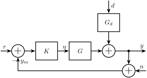
Figure 1: Block Diagram of a simple feedback system
Without the use of feedback (i.e. without the nano-hexapod), the disturbances will induce a sample motion error equal to:
\begin{equation} y = G_d d \label{eq:open_loop_error} \end{equation}which is, in the case of the NASS out of the specifications (micro-meter range compare to the required \(\approx 10nm\)).
In the next section, is explained how the use of the feedback lowers the effect of the disturbances \(d\) on the sample motion error.
1.1.2 How does the feedback loop is modifying the system behavior?
From the feedback diagram in Figure 1, the position error signal \(\epsilon = r - y\) can be written as a function of the reference signal \(r\), the disturbances \(d\) and the measurement noise \(n\): \[ \epsilon = \frac{1}{1 + GK} r + \frac{GK}{1 + GK} n - \frac{G_d}{1 + GK} d \]
It is common to define the following two transfer functions:
\begin{align} S &= \frac{1}{1 + GK} \\ T &= \frac{GK}{1 + GK} \end{align}where \(S\) is called the sensitivity transfer function and \(T\) the transmissibility (or complementary sensitivity) transfer function.
And the position error can be rewritten as:
\begin{equation} \epsilon = S r + T n - G_d S d \label{eq:closed_loop_error} \end{equation}From Eq. \eqref{eq:closed_loop_error} representing the closed-loop system behavior, it is seen that:
- the effect of disturbances \(d\) on \(\epsilon\) is multiplied by a factor \(S\) compared to the open-loop case
- the measurement noise \(n\) is injected and multiplied by a factor \(T\)
Ideally, it is desired to design the controller \(K\) such that:
- \(|S|\) is small to reduce the effect of disturbances
- \(|T|\) is small to limit the injection of sensor noise
1.1.3 Trade off: Disturbance Reduction / Noise Injection
From the definition of \(S\) and \(T\):
\begin{equation} S + T = \frac{1}{1 + GK} + \frac{GK}{1 + GK} = 1 \end{equation}meaning that it is not possible to have \(|S|\) and \(|T|\) small at the same time.
There is therefore a trade-off between the disturbance rejection and the measurement noise filtering.
Typical shapes of \(|S|\) and \(|T|\) as a function of frequency are shown in Figure 2. It is shown that \(|S|\) and \(|T|\) exhibit different behaviors depending on the frequency band:
- At low frequency (inside the control bandwidth):
- \(|S|\) can be made small and thus the effect of disturbances is reduced
- \(|T| \approx 1\) and all the sensor noise is transmitted
- At high frequency (outside the control bandwidth):
- \(|S| \approx 1\) and the feedback system does not reduce the effect of disturbances
- \(|T|\) is small and thus the sensor noise is filtered
- Near the crossover frequency (between the two frequency bands):
- The effect of disturbances is increased
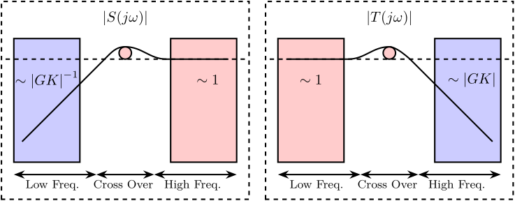
Figure 2: Typical shapes and constrain of the Sensitivity and Transmibility closed-loop transfer functions
1.1.4 Trade off: Robustness / Performance
As shown in the previous section, the effect of disturbances is reduced inside the control bandwidth.
Moreover, the slope of \(|S(j\omega)|\) is limited for stability reasons (not explained here), and therefore a large control bandwidth is required to obtain sufficient disturbance rejection at lower frequencies (where the disturbances have usually large effects).
The next important question is therefore what limits the attainable control bandwidth?
The main issue it that for stability reasons, the system dynamics must be known with only small uncertainty in the vicinity of the crossover frequency.
For mechanical systems, this generally means that the control bandwidth should take place before any appearing of flexible dynamics (right part of Figure 3).
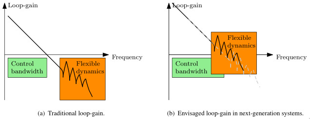
Figure 3: Envisaged developments in motion systems. In traditional motion systems, the control bandwidth takes place in the rigid-body region. In the next generation systemes, flexible dynamics are foreseen to occur within the control bandwidth. oomen18_advan_motion_contr_precis_mechat
This also means that any possible change in the system should have a small impact on the system dynamics in the vicinity of the crossover.
For the NASS, the possible changes in the system are:
- a modification of the payload mass and dynamics
- a change of experimental condition: spindle’s rotation speed, position of each micro-station’s stage
- a change in the micro-station dynamics (change of mechanical elements, aging effect, …)
The nano-hexapod and the control architecture have to be developed in such a way that the feedback system remains stable and exhibit acceptable performance for all these possible changes in the system.
This problem of robustness represent one of the main challenge for the design of the NASS.
1.2 Dynamic error budgeting
The dynamic error budgeting is a powerful tool to study the effects of multiple error sources (i.e. disturbances and measurement noise) and to predict how much these effects are reduced by a feedback system.
The dynamic error budgeting uses two important mathematical functions: the Power Spectral Density and the Cumulative Power Spectrum.
After these two functions are introduced (in Sections 1.2.1 and 1.2.2), is shown how do multiple error sources are combined and modified by dynamical systems (in Section 1.2.3 and 1.2.4).
Finally, the dynamic noise budgeting for the NASS is derived in Section 1.2.5.
1.2.1 Power Spectral Density
The Power Spectral Density (PSD) \(S_{xx}(f)\) of the time domain signal \(x(t)\) is defined as the Fourier transform of the autocorrelation function: \[ S_{xx}(\omega) = \int_{-\infty}^{\infty} R_{xx}(\tau) e^{-j \omega \tau} d\tau \quad \frac{[\text{unit of } x]^2}{\text{Hz}} \]
The PSD \(S_{xx}(\omega)\) represents the distribution of the (average) signal power over frequency.
Thus, the total power in the signal can be obtained by integrating these infinitesimal contributions. The Root Mean Square (RMS) value of the signal \(x(t)\) is then:
\begin{equation} x_{\text{rms}} = \sqrt{\int_{0}^{\infty} S_{xx}(\omega) d\omega} \end{equation}One can also integrate the infinitesimal power \(S_{xx}(\omega)d\omega\) over a finite frequency band to obtain the power of the signal \(x\) in that frequency band:
\begin{equation} P_{f_1,f_2} = \int_{f_1}^{f_2} S_{xx}(\omega) d\omega \quad [\text{unit of } x]^2 \end{equation}1.2.2 Cumulative Power Spectrum
The Cumulative Power Spectrum is the cumulative integral of the Power Spectral Density starting from \(0\ \text{Hz}\) with increasing frequency:
\begin{equation} CPS_{+_x}(f) = \int_0^f S_{xx}(\nu) d\nu \quad [\text{unit of } x]^2 \end{equation}The Cumulative Power Spectrum \(CPS_{+}\) taken at frequency \(f\) thus represent the power in the signal in the frequency band \(0\) to \(f\).
An alternative definition of the Cumulative Power Spectrum can be used where the PSD is integrated from \(f\) to \(\infty\):
\begin{equation} CPS_{-_x}(f) = \int_f^\infty S_{xx}(\nu) d\nu \quad [\text{unit of } x]^2 \end{equation}And thus \(CPS_{-_x}(f)\) represents the power in the signal \(x\) for frequencies above \(f\).
The Cumulative Power Spectrum is generally shown as a function of frequency, and is used to identify the critical modes in a design, at which the effort should be targeted. It can also helps to determine at which frequencies the effect of disturbances must be reduced, and thus the approximate required control bandwidth.
A typical Cumulative Power Spectrum is shown in figure 4.
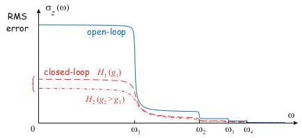
Figure 4: Cumulative Power Spectrum \(CPS_{-}\) in open-loop and closed-loop for increasing gains (taken from preumont18_vibrat_contr_activ_struc_fourt_edition)
1.2.3 Modification of a signal’s PSD when going through a dynamical system
Let’s consider a signal \(u\) with a PSD \(S_{uu}\) going through a LTI system \(G(s)\) that outputs a signal \(y\) with a PSD (Figure 5).

Figure 5: LTI dynamical system \(G(s)\) with input signal \(u\) and output signal \(y\)
The Power Spectral Density of the output signal \(y\) can be computed using:
\begin{equation} S_{yy}(\omega) = \left|G(j\omega)\right|^2 S_{uu}(\omega) \end{equation}1.2.4 PSD of combined signals
Let’s consider a signal \(y\) that is the sum of two uncorrelated signals \(u\) and \(v\) (Figure 6).
The PSD of \(y\) is equal to sum of the PSD and \(u\) and the PSD of \(v\) (can be easily shown from the definition of the PSD): \[ S_{yy} = S_{uu} + S_{vv} \]
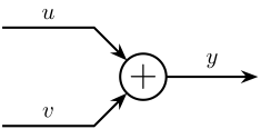
Figure 6: \(y\) as the sum of two signals \(u\) and \(v\)
1.2.5 Dynamic Noise Budgeting
Let’s consider the Feedback architecture in Figure 1 where the position error \(\epsilon\) is equal to: \[ \epsilon = S r + T n - G_d S d \]
Supposing that the signals \(r\), \(n\) and \(d\) are uncorrelated (which is a good approximation in our case), the PSD of \(\epsilon\) is equal to: \[ S_{\epsilon \epsilon}(\omega) = |S(j\omega)|^2 S_{rr}(\omega) + |T(j\omega)|^2 S_{nn}(\omega) + |G_d(j\omega) S(j\omega)|^2 S_{dd}(\omega) \]
And the RMS value of the residual motion can be computed using:
\begin{align*} \epsilon_\text{rms} &= \sqrt{ \int_0^\infty S_{\epsilon\epsilon}(\omega) d\omega} \\ &= \sqrt{ \int_0^\infty \Big( |S(j\omega)|^2 S_{rr}(\omega) + |T(j\omega)|^2 S_{nn}(\omega) + |G_d(j\omega) S(j\omega)|^2 S_{dd}(\omega) \Big) d\omega } \end{align*}To estimate the PSD of the position error \(\epsilon\) and thus the RMS residual motion (in closed-loop), the following needs to be determined:
- The Power Spectral Densities of the signals affecting the system:
- The disturbances \(S_{dd}\): this will be done in Section 3
- The sensor noise \(S_{nn}\): this can be estimated from the sensor data-sheet
- The wanted sample’s motion \(S_{rr}\): this is a deterministic signal that is chosen by the “user”. For a simple tomography experiment, the wanted sample’s motion can consider to be equal to \(0\) (the point of interest should stay on the focus X-ray)
- The dynamics of the complete system comprising the micro-station and the nano-hexapod: \(G\), \(G_d\). To do so, the dynamics of the micro-station (Section 2) should be identified and then included in a model (Section 4). Then a model of the nano-hexapod is merged with the micro-station model (Section 5)
- The controller \(K\) that will be designed in Section 6
2 Identification of the Micro-Station Dynamics
As explained before, it is very important to have a good estimation of the micro-station dynamics as it will be used:
- to tune the developed multi-body model of the micro-station with which the simulations will be performed
- for the design of the nano-hexapod as it will be coupled with the micro-station
- for the design of the controller
All the measurements performed on the micro-station are detailed in this document and summarized in the following sections.
The general procedure to identify the dynamics of the micro-station is shown in Figure 7. The steps are:
- extract a Response Model (Frequency Response Functions) from measurements
- convert the Response Model into a Modal Model (Natural Frequencies and Mode Shapes)
- extract a Spatial Model from the Modal Model (Mass/Damping/Stiffness matrices)
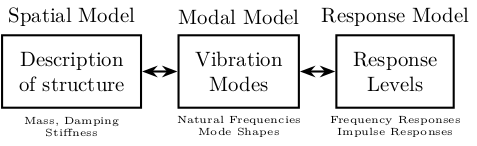
Figure 7: Vibration Analysis Procedure
The extraction of the Spatial Model (3rd step) was not performed as it requires a lot of time and was not judge necessary. Instead, the model will be tuned using both the modal model and the response model.
2.1 Experimental Setup
To measure the dynamics of such complicated system, it as been chosen to perform a modal analysis.
To limit the number of degrees of freedom to be measured, it is supposed that in the frequency range of interest (DC-300Hz), each of the positioning stage is behaving as a solid body. Thus, to fully describe the dynamics of the station, only 6 degrees of freedom for each positioning stage (that is 36 degrees of freedom for the 6 considered solid bodies) should be measured.
In order to perform the modal analysis, the following devices were used:
- An acquisition system (OROS) with 24bits ADCs
- 3 tri-axis Accelerometers
- An Instrumented Hammer
The measurement consists of:
- Exciting the structure at the same location with the instrumented hammer (Figure 8)
- Fix the accelerometers on each of the stages to measure all the DOF of the structure.
The position of the accelerometers are:
- 4 on the first granite
- 4 on the second granite
- 4 on top of the translation stage (Figure 9)
- 4 on top of the tilt stage
- 3 on top of the spindle
- 4 on top of the hexapod
In total, 69 degrees of freedom are measured (23 tri axis accelerometers) which is more that what was required.
It was chosen to have some redundancy in the measurement to be able to verify the correctness of the solid-body assumption.
Figure 8: Example of one hammer impact
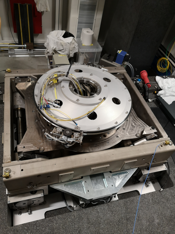
Figure 9: 3 tri axis accelerometers fixed to the translation stage
2.2 Results
From the measurements are extracted all the transfer functions from forces applied at the location of the hammer impacts to the x-y-z acceleration of each solid body at the location of each accelerometer.
Modal shapes and natural frequencies are then computed. Example of the obtained micro-station’s mode shapes are shown in Figures 10 and 11.
Figure 10: First mode that shows a suspension mode, probably due to bad leveling of one Airloc
Figure 11: Sixth mode
The number of degrees of freedom is then reduced from 69 (23 accelerometers with each 3DOF) down to 36 (6 solid bodies with 6 DOF).
From the reduced transfer function matrix, the responses at the 69 measured degrees of freedom are re-synthesized. The original measurements and the synthesized one are compared and found to match.
This confirms the fact that the stages are indeed behaving as a solid body in the frequency band of interest.
This thus means that a multi-body model can be used to correctly represent the dynamics of the micro-station.
Many Frequency Response Functions (FRF) are obtained from the measurements. Examples of FRF are shown in Figure 12. These FRF will be used to compare the dynamics of the multi-body model with the micro-station dynamics.
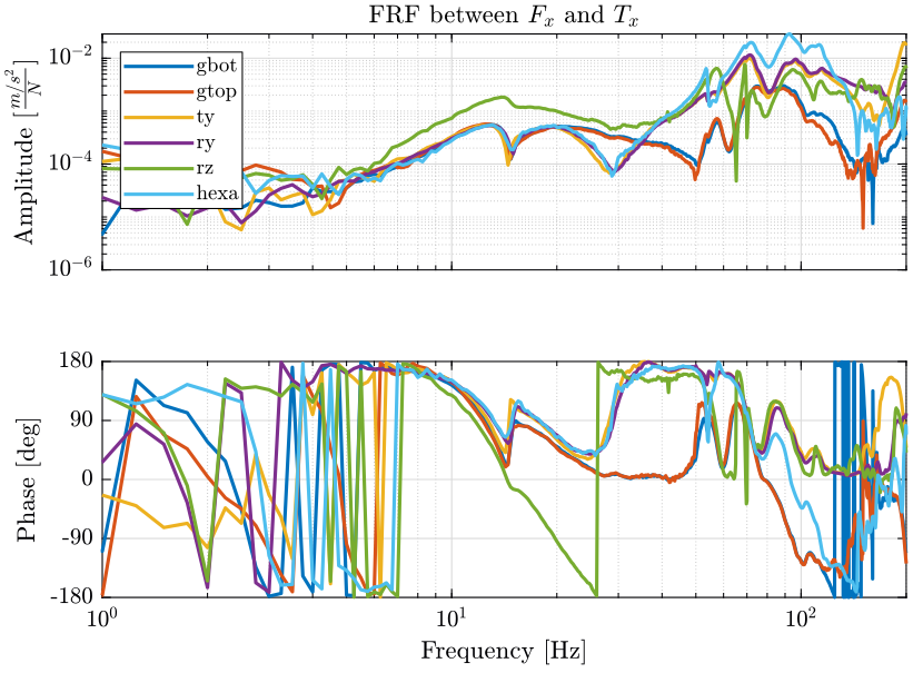
Figure 12: Frequency Response Function from forces applied by the Hammer in the X direction to the acceleration of each solid body in the X direction
2.3 Conclusion
The dynamical measurements made on the micro-station confirmed the fact that a multi-body model is a good option to correctly represents the micro-station dynamics.
In Section 4, the obtained Frequency Response Functions will be used to compare the model dynamics with the micro-station dynamics.
3 Identification of the Disturbances
In this section, all the disturbances affecting the system are identified and quantified.
Note that the low frequency disturbances such as static guiding errors and thermal effects are not much of interest here, because the frequency content of these errors will be located way inside the controller bandwidth and thus will be easily compensated by the nano-hexapod. These are however very important for the evaluation of the required nano-hexapod mobility and will be identified separately.
The main challenge is to reduce the disturbances containing high frequencies, and thus efforts are made to identify these high frequency disturbances such as:
- Ground motion (Section 3.1)
- Vibration introduced by control systems (Section 3.2)
- Vibration introduced by the motion of the spindle and of the translation stage (Section 3.3)
A noise budgeting is performed in Section 3.4, the vibrations induced by the disturbances are compared and the required control bandwidth is estimated.
The measurements are presented in more detail in this document and the open loop noise budget is done in this document.
3.1 Ground Motion
Ground motion can easily be estimated using an inertial sensor with sufficient resolution.
To verify that the inertial sensors are sensitive enough, a Huddle test has been performed (Figure 13). The details of the Huddle Test can be found here.
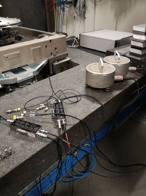
Figure 13: Huddle Test Setup
The measured Power Spectral Density of the ground motion at the ID31 floor is compared with other measurements performed at ID09 and at CERN. The low frequency differences between the ground motion at ID31 and ID09 is just due to the fact that for the later measurement, the low frequency dynamics of the inertial sensor was not taken into account.
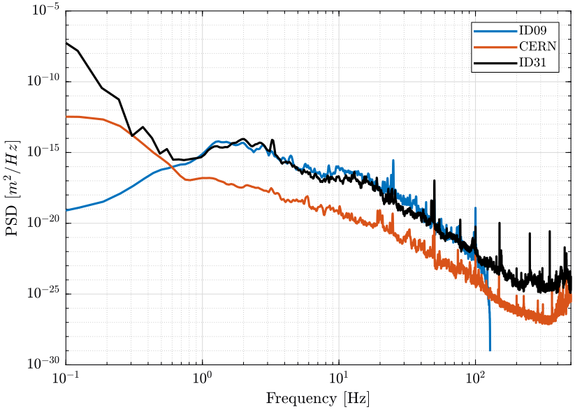
Figure 14: Comparison of the PSD of the ground motion measured at different location
3.2 Stage Vibration - Effect of Control systems
The effect of the control system of each micro-station’s stage is identified.
To do so, one geophone is located at the sample’s location which another is located on the granite. The feedback loop of each stage is turned on and off, and the vibrations level of the sample with respect to the granite is measured. Note that here no stage is performing motion, just the disturbances introduced by the feedback loops are identified.
It is shown that these local feedback loops have little influence on the sample’s vibrations except the Spindle that introduced a sample’s vertical motion at 25Hz.
Complete reports on these measurements are accessible here and here.
3.3 Stage Vibration - Effect of Motion
In this section, the vibrations induced by scans of the translation stage and rotation of the spindle and studied.
Details reports are accessible here for the translation stage and here for the spindle/slip-ring.
Spindle and Slip-Ring
The setup for the measurement of vibrations induced by rotation of the Spindle and Slip-ring is shown in Figure 15.
Figure 15: Measurement of the sample’s vertical motion when rotating at 6rpm
A geophone is fixed at the location of the sample and the motion is measured:
- without any rotation
- when rotating at 6rpm using only the slip-ring motor
- when rotating at 6rpm using the spindle motor synchronized with the slip-ring motor
The obtained Power Spectral Densities of the sample’s absolute velocity are shown in Figure 16.
It can be seen that when using the Slip-ring motor to rotate the sample, only a little increase of the motion is observed above 100Hz.
However, when rotating with the Spindle (normal functioning mode):
- a very sharp peak at 23Hz is observed. Its cause has not been identified yet
- a general large increase in motion above 30Hz
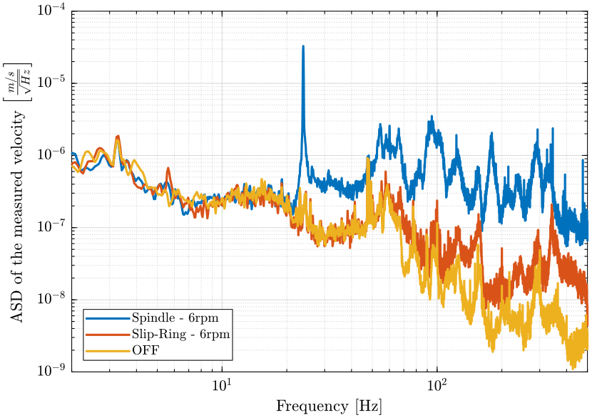
Figure 16: Comparison of the ASD of the measured voltage from the Geophone at the sample location
Some investigation should be performed to determine where does this 23Hz motion comes from and why such high frequency motion is introduced by the spindle’s motor.
Translation Stage
The same setup is used: a geophone is located at the sample’s location and another on the granite.
A 1Hz triangle motion with an amplitude of \(\pm 2.5mm\) is sent to the translation stage (Figure 17), and the absolute velocities of the sample and the granite are measured.
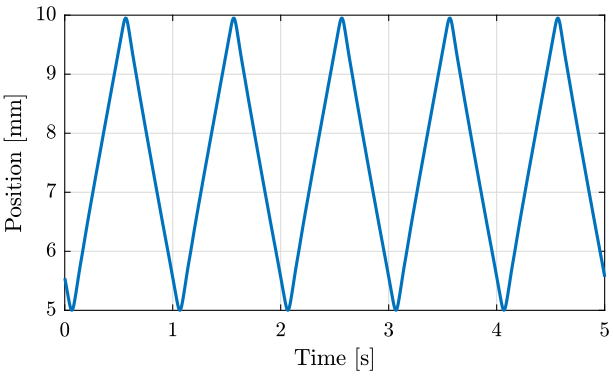
Figure 17: Y position of the translation stage measured by the encoders
The time domain absolute vertical velocity of the sample and granite are shown in Figure 18. It is shown that quite large motion of the granite is induced by the translation stage scans. This could be a problem if this is shown to excite the metrology frame of the nano-focusing lens position stage.
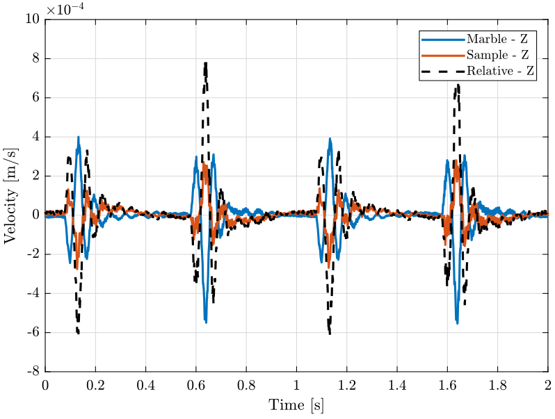
Figure 18: Vertical velocity of the sample and marble when scanning with the translation stage
The Amplitude Spectral Densities of the measured absolute velocities are shown in Figure 19. The ASD contains any peaks starting from 1Hz showing the large spectral content of the motion which is probably due to the triangular reference of the translation stage.
A smoother motion for the translation stage (such as a sinus motion, of a filtered triangular signal) could help reducing much of the vibrations. The goal is to inject no motion outside the control bandwidth.
It should be noted that away from the rapid change of velocity, the sample’s vibrations are much reduced. Thus, if the detector is only used in between the triangular peaks, the vibrations are expected to be much lower than those estimated.
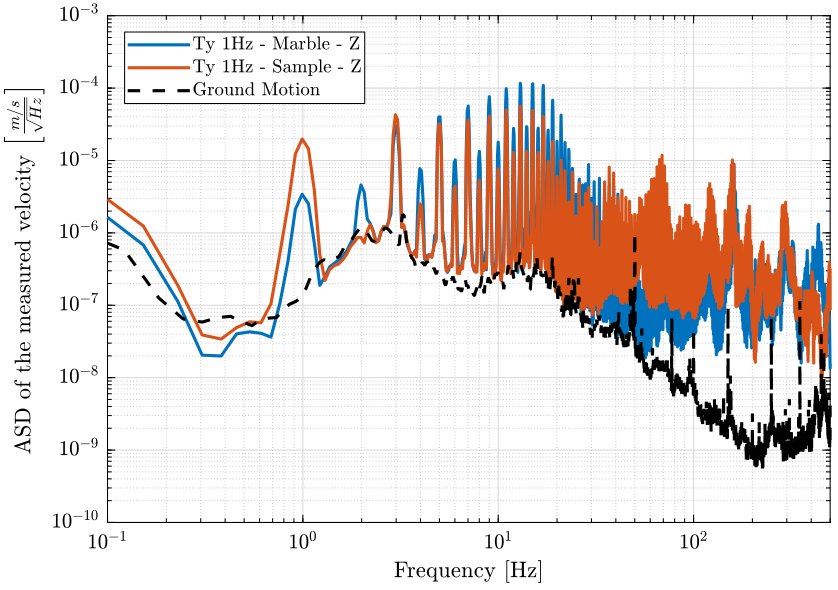
Figure 19: Amplitude spectral density of the measure velocity corresponding to the geophone in the vertical direction located on the granite and at the sample location when the translation stage is scanning at 1Hz
3.4 Open Loop noise budgeting
The effect of all the disturbance sources on the position error (relative motion of the sample with respect to the granite) are now compared.
The Power Spectral Density of the motion error due to the ground motion, translation stage scans and spindle rotation are shown in Figure 20.
It can be seen that the ground motion is quite small compare to the translation stage and spindle induced motions.
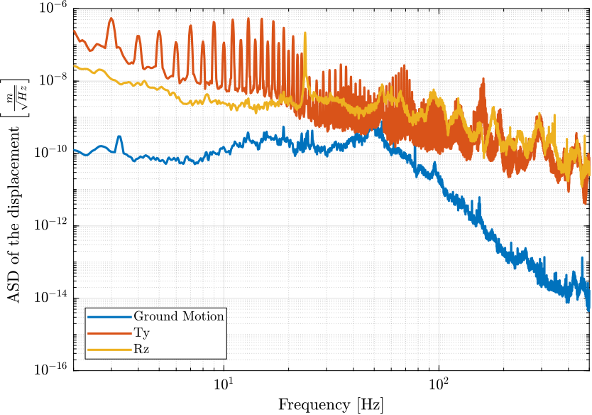
Figure 20: Amplitude Spectral Density fo the motion error due to disturbances
The Cumulative Amplitude Spectrum is shown in Figure 21. It is shown that the motion induced by translation stage scans and spindle rotation are in the micro-meter range for frequencies above 1Hz.
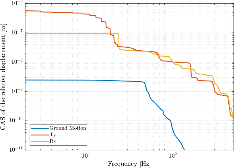
Figure 21: Cumulative Amplitude Spectrum \(CAS_{-}\) of the motion error due to disturbances
From Figure 21, required bandwidth can be estimated by seeing that \(10\ nm [rms]\) motion is induced by the perturbations above 100Hz.
This means that if the controller compensate all the motion errors below 100Hz (ideal case), 10nm [rms] of motion will still remain.
From that, it can be concluded that control bandwidth will have to be around 100Hz.
3.5 Better estimation of the disturbances
All the disturbance measurements were made with inertial sensors, and to obtain the relative motion sample/granite, two inertial sensors were used and the signals were subtracted.
This is not perfect as using only one geophone on the sample and one on the granite do not permit to separate translations and rotations.
An alternative could be to position a small calibrated sphere at the sample location and to use the X-ray to measure its motion while performing translation scans and spindle rotations.
The detector requirement would need to have a sample frequency above \(400Hz\) and a resolution of \(\approx 100nm\) (to be discussed).
3.6 Conclusion
Main disturbance sources have been identified (ground motion, vibrations of the translation stage and the spindle). These disturbances will then be included in the multi-body model.
Other disturbance sources were not estimated such as cable forces and acoustic disturbances. If heavy/stiff cables are to be fixed to the sample, this should be quantified and included in the model.
A better estimation of the disturbances would allow a more precise estimation the attainable performance. This should however not change the conclusion of this study nor significantly change the nano-hexapod design.
4 Multi Body Model
As was shown during the modal analysis (Section 2), the micro-station behaves as multiple rigid bodies (granite, translation stage, tilt stage, spindle, hexapod) connected with some discrete flexibility (stiffnesses and dampers).
Thus, a multi-body model is perfectly adapted to represent the dynamics of the micro-station.
The Matlab’s Simscape toolbox is used to develop the multi-body model. A small summary of the multi-body Simscape is available here and each of the modeled stage is described here.
4.1 Multi-Body model
The parameters to tune the dynamics of the multi body are:
- the mass/moment of inertia of each of the solid bodies
- the 6 stiffnesses and 6 damping properties representing each of the the mechanical guiding between two solid bodies
The mass/inertia of each stage is automatically computed from the imported geometry and the material’s density.
The stiffnesses between two solid bodies is first guessed from either measurements of data-sheets. Then, the values of the stiffnesses and damping properties of each joint is manually tuned until the obtained dynamics is sufficiently close to the measured dynamics.
The 3D representation of the simscape model is shown in Figure 22.
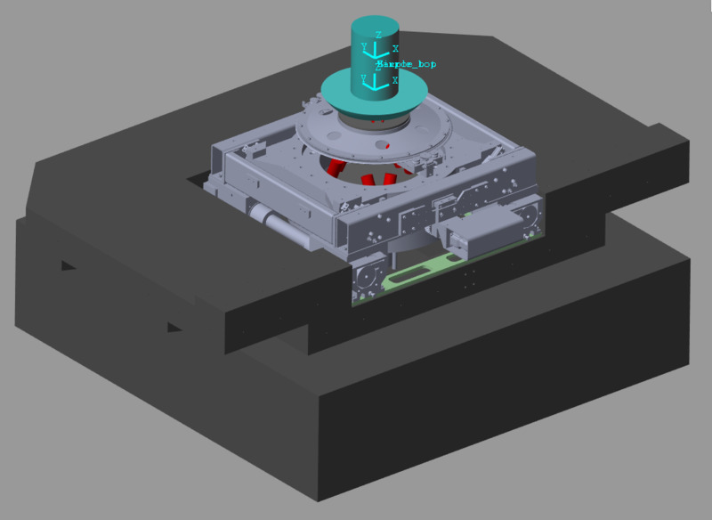
Figure 22: 3D representation of the simscape model
4.2 Validity of the model’s dynamics
Tuning the dynamics of such model is very difficult as there are more than 50 parameters to tune and many different dynamics to compare between the model and the measurements.
The comparison of three of the Frequency Response Functions are shown in Figure 23.
Most of the other measured FRFs and identified transfer functions from the multi-body model have the same level of matching.
We believe that the model is representing the micro-station dynamics sufficient well for the current analysis.
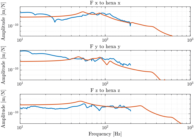
Figure 23: Frequency Response function from Hammer force in the X,Y and Z directions to the X,Y and Z displacements of the micro-hexapod’s top platform. The measurements are shown in blue and the Model in red.
More detailed comparison between the model and the measured dynamics is performed here.
Now that the multi-body model dynamics has been tuned, the following elements are included:
- Actuators to perform the motion of each stage (translation, tilt, spindle, hexapod)
- Sensors to measure the motion of each stage and the relative motion of the sample with respect to the granite (metrology system)
- Disturbances such as ground motion and stage’s vibrations
Then, using the model, it is possible to:
- perform simulation of experiments in presence of disturbances
- measure the motion of the solid-bodies
- identify the dynamics from inputs (forces, imposed displacement) to outputs (measured motion, force sensor, etc.) which will be useful for the nano-hexapod design and the control synthesis
- include a multi-body model of the nano-hexapod and perform closed-loop simulations
4.3 Wanted position of the sample and position error
For the control of the nano-hexapod, the sample position error (the motion to be compensated) in the frame of the nano-hexapod needs to be computed.
To do so, several computations are performed (summarized in Figure 24):
- First, the wanted pose (3 translations and 3 rotations) of the sample with respect to the granite is computed. This is determined from the wanted motion of each micro-station stage: each wanted stage motion is represented by a homogeneous transformation matrix that are combined to give to total wanted motion of the sample with respect to the granite
- Then, the actual pose of the sample with respect to the granite is computed. For the real system, this will require the use of several interferometers and computations to obtain the sample’s pose from the individual measurements. However, the pose of the sample with respect to the granite is directly measured using a special simscape block
- Finally, the wanted pose is compared with the measured pose to compute the position error of the sample. This position error can be expressed in the frame of the granite, or in the frame of the (rotating) nano-hexapod. Both computation are performed
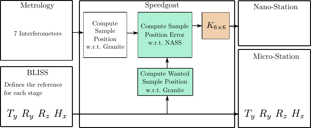
Figure 24: Schematic of how the elements are interacting with the Speedgoat
More details about these computations are accessible here.
4.4 Simulation of a Tomography Experiment
Now that the dynamics of the model is tuned and the disturbances included in the model, simulations of experiments can be performed.
A first simulation is done with the nano-hexapod modeled as a rigid-body. This does represent the system without the NASS and permits to estimate the sample’s vibrations using the micro-station alone. The results of this simulation will be compared to simulations using the NASS in Section 6.4.
An 3D animation of the simulation is shown in Figure 25.
A zoom in the micro-meter ranger on the sample’s location is shown in Figure 26 with two frames:
- a non-rotating frame corresponding to the focusing point of the X-ray. It does in that case correspond to the wanted position of the sample. Note that this frame is moving with the granite as the nano-focusing optics are fixed to the granite.
- a rotating frame that corresponds to the actual pose of the sample
The motion of the sample follows the wanted motion but with vibrations in the micro-meter range as was expected.
Figure 25: Tomography Experiment using the Simscape Model

Figure 26: Tomography Experiment using the Simscape Model - Zoom on the sample’s position (the full vertical scale is \(\approx 10 \mu m\))
The position error of the sample with respect to the granite are shown in Figure 27. It is confirmed that the X-Y-Z position errors are in the micro-meter range.
For the rotation around X and Y, the errors are quite small. This is explained by the fact that no torque disturbances is considered in the model.
The vertical rotation error is meaningless for two reasons:
- the rotation of the Spindle is considered to be perfect
- no measurement of the sample’s vertical rotation with respect to the granite is made by the interferometers
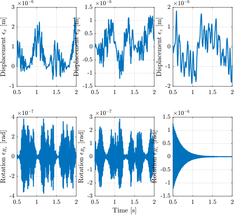
Figure 27: Position error of the Sample with respect to the granite during a Tomography Experiment with included disturbances
4.5 Conclusion
The multi-body model has been tuned to represents the micro-station dynamics and includes disturbances such as ground motion and stages vibrations.
It can be used to:
- study many effects such as the change of dynamics due to the rotation, the sample mass, etc.
- extract transfer function like plant dynamics \(G\) and sensibility to disturbances \(G_d\)
- simulate experiments
In the next sections, it will allows to optimally design the nano-hexapod, to develop a robust control architecture and to perform simulations to estimate the system’s performances.
5 Optimal Nano-Hexapod Design
As explain before, the nano-hexapod properties (mass, stiffness, legs’ orientation, …) will influence:
- the effect of disturbances
- the plant dynamics
The objective is here to find the optimal nano-hexapod properties such that:
- the effect of disturbances is minimized (Section 5.2)
- the plant uncertainty due to a change of payload mass and experimental conditions is minimized (Section 5.3)
- the plant has nice dynamical properties for control (Section 5.4)
In this study, the effect of the nano-hexapod’s mass characteristics is not taken into account because it cannot be changed a lot and it is quite negligible compare the to metrology reflector and the payload’s masses that are fixed to nano-hexapod’s top platform.
Also, the nano-hexapod’s damping is not studied here as it is supposed to be very small, and active damping techniques will be included in the control architecture to add the wanted amount of damping.
5.1 A brief introduction to Stewart Platforms
A typical Stewart platform is composed of two platforms connected by six identical struts (or legs) composed of:
- a universal joint at one end
- a spherical joint at the other end
- a prismatic joint with an associated actuator
This is very schematically shown in Figure 28 where the \(a_i\) are the location of the joints connected to the fixed platform and the \(b_i\) are the joints connected to the mobile platform.
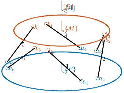
Figure 28: Schematic representation of a Stewart platform
As shows in Figure 28, two frames \(\{A\}\) and \(\{B\}\) are virtually fixed to respectively the bottom and the top platforms. These frames are used to describe the relative motion of the two platforms through the position vector \({}^A\bm{P}_B\) of \(\{B\}\) expressed in \(\{A\}\) and the rotation matrix \({}^A\bm{R}_B\) expressing the orientation of \(\{B\}\) with respect to \(\{A\}\). For the nano-hexapod, these frames are chosen to be located at the theoretical center of the spherical metrology reflector.
Since the Stewart platform has six-degrees-of-freedom and six actuators, it is called a fully parallel manipulator. A change in the length of the legs \(\bm{\mathcal{L}} = \left[ l_1, l_2, l_3, l_4, l_5, l_6 \right]^T\) will induce a motion of the mobile platform with respect to the fixed platform as shown in Figure 29. The relation between a change in length of the legs and the relative motion of the platforms is studied thanks to the kinematic analysis, which is explained in Section 5.4.
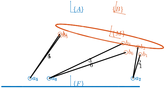
Figure 29: Display of the Stewart platform architecture at some defined pose
The Stewart Platform is very adapted for the NASS application for the following reasons:
- it is a fully parallel manipulator, thus all the motions errors can be compensated
- it is very compact compared to a serial manipulator
- it has high stiffness and good dynamic performances
The main disadvantage of Stewart platforms is the small workspace when compare the serial manipulators which is not a problem here.
A Matlab toolbox to study and design Stewart Platforms has been developed and used for the design of the nano-hexapod. The source code is accessible here and the documentation here.
Extensive analysis of parallel manipulator, and in particular the Stewart platform is given in [4].
5.2 Optimal Stiffness to reduce the effect of disturbances
As will be seen, the nano-hexapod stiffness have a large influence on the sensibility to disturbance (the norm of \(G_d\)). For instance, it is quite obvious that a stiff nano-hexapod is better than a soft one when it comes to direct forces applied to the sample such as cable forces.
A study of the optimal nano-hexapod stiffness for the minimization of disturbance sensibility is accessible here and summarized below.
Sensibility to stage vibrations
The sensibility to the spindle’s vibration for all the considered nano-hexapod stiffnesses (from \(10^3\,[N/m]\) to \(10^9\,[N/m]\)) is shown in Figure 30. It is shown that a softer nano-hexapod is better to filter out vertical vibrations of the spindle. More precisely, the nano-hexapod filters out the vibration starting at the first suspension mode of the payload on top of the nano-hexapod.
The same conclusion is made for vibrations of the translation stage.
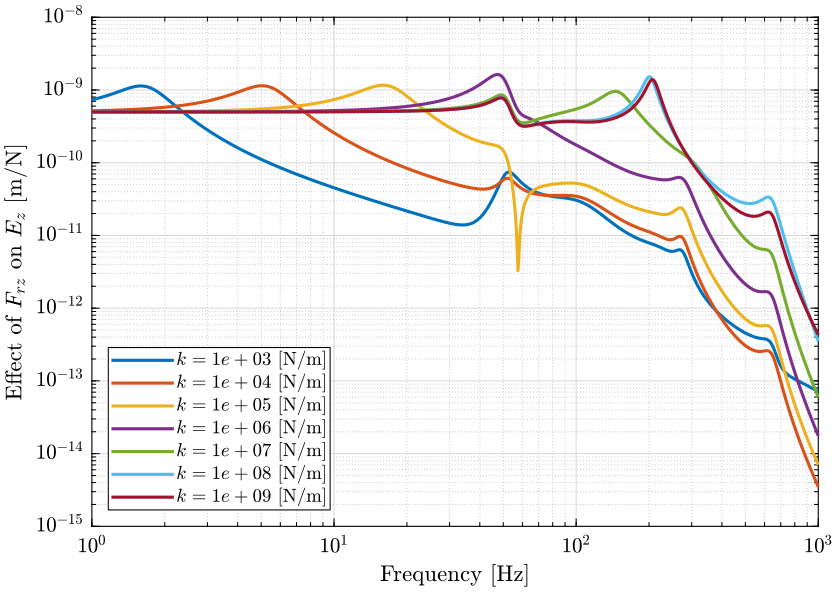
Figure 30: Sensibility to Spindle vertical motion error to the vertical error position of the sample
Sensibility to ground motion
The sensibility to ground motion in the Y and Z directions is shown in Figure 31. Above the suspension mode of the nano-hexapod, the norm of the transmissibility is close to one until the suspension mode of the granite. Thus, a stiff nano-hexapod (\(k>10^5\,[N/m]\)) is better for reducing the effect of ground motion at low frequency.
It will be suggested in Section 7.6 that using soft mounts for the granite can greatly lower the sensibility to ground motion.
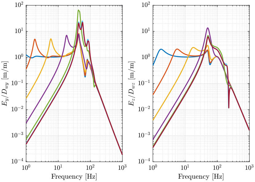
Figure 31: Sensibility to Ground motion to the position error of the sample
Dynamic Noise Budgeting considering all the disturbances
Looking at the change of sensibility with the nano-hexapod’s stiffness helps understand the physics of the system. It however, does not permit to estimate the optimal stiffness that will lower the motion error due to disturbances.
To do so, the power spectral density of the disturbances should be taken into account, as the sensibility of one disturbance should be reduced only where the PSD of the considered disturbance is large compared to the other disturbances.
What is more important than comparing the sensitivity to disturbances, is to compare the resulting open-loop power spectral density of the sample’s position error with the change of the nano-hexapod’s stiffness. This is the dynamic noise budgeting.
From the Power Spectral Density of all the sources of disturbances identified in Section 3 is computed the Power Spectral Density of the vertical motion error for all the considered nano-hexapod stiffnesses (Figure 32).
It can be seen that the most important change is in the frequency range 30Hz to 300Hz where a stiffness smaller than \(10^5\,[N/m]\) greatly reduces the sample’s vibrations.
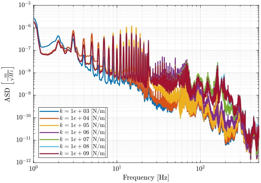
Figure 32: Amplitude Spectral Density of the Sample vertical position error due to Vertical vibration of the Spindle for multiple nano-hexapod stiffnesses
Conclusion
It can be observe on the Cumulative amplitude spectrum of the vertical error motion in Figure 33, that a soft hexapod (\(k < 10^5 - 10^6\,[N/m]\)) helps reducing the high frequency disturbances, and thus a smaller control bandwidth will be required to obtain the wanted performance.
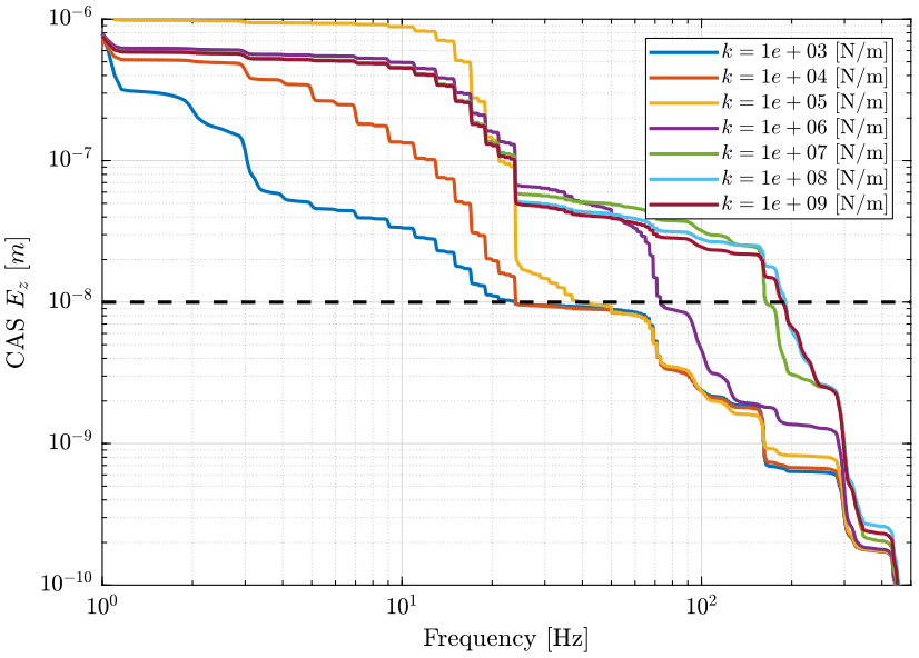
Figure 33: Cumulative Amplitude Spectrum \(CAS_{-}\) of the Sample vertical position error due to all considered perturbations for multiple nano-hexapod stiffnesses. The dashed back line corresponds to the wanted \(10nm\,rms\) of residual motion.
5.3 Optimal Stiffness to reduce the plant uncertainty
One of the most important design goal is to obtain a system that is robust to all changes in the system. Therefore, all changes that might occur in the system must be identified and the nano-hexapod stiffness that minimizes the uncertainties to these changes should be determined.
The uncertainty in the system can be caused by:
- A change in the Support’s compliance (complete analysis here): if the micro-station dynamics is changing due to the change of mechanical parts or just because of aging effects, the feedback system should remains stable and the obtained performance should not change
- A change in the Payload mass/dynamics (complete analysis here): the sample’s mass is ranging from \(1\,kg\) to \(50\,kg\)
- A change of experimental condition such as the micro-station’s pose or the spindle rotation speed (complete analysis here)
Because of the trade-off between robustness and performance, the bigger the plant dynamic uncertainty, the lower the attainable performance will be for all the system changes.
In the next sections, the effect the considered changes on the plant dynamics is quantified and conclusions are drawn on the optimal stiffness for robustness properties.
In the following study, when it is referred to plant dynamics, it means the dynamics from forces applied by the nano-hexapod to the measured sample’s displacement by the metrology. Only the plant dynamics will be compared as it is the most important dynamics for robustness and performance properties. However, the dynamics from forces to sensors located in the nano-hexapod legs, such as force and relative motion sensors, have also been considered in a separate study.
Effect of Payload
The most obvious change in the system is the change of payload.
In Figure 34 the dynamics is shown for payloads with a mass equal to 1kg, 20kg and 50kg (the resonance of the payload is fixed to 100Hz). On the left side, the change of dynamics is computed for a very soft nano-hexapod, while on the right side, it is computed for a very stiff nano-hexapod.
One can see that for the soft nano-hexapod:
- the first resonance (suspension mode of the nano-hexapod) is lowered with an increase of the sample’s mass. This is very logical as the first resonance corresponds to \(\omega = \sqrt{\frac{k_n}{m_n + m_s}}\) where \(k_n\) is the vertical nano-hexapod stiffness, \(m_n\) the mass of the nano-hexapod’s top platform, and \(m_s\) the sample’s mass
- the gain after the first resonance and up until the anti-resonance at 100Hz is changing with the sample’s mass. It is indeed equal to \(\frac{1}{(m_n + m_s) \omega^2}\)
For the stiff-nano-hexapod, the change of payload mass has very little effect (the vertical scale for the amplitude is quite small).
To minimize the uncertainty to the payload’s mass, the mass of the nano-hexapod’s top platform plus the metrology reflector should be maximized, and ideally close to the maximum payload’s mass. As the maximum payload’s mass is \(50\,kg\), this may however not be practical, and thus the control architecture must be developed to be robust to a change of the payload’s mass.
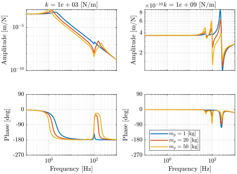
Figure 34: Dynamics from \(\mathcal{F}_z\) to \(\mathcal{X}_z\) for varying payload mass, both for a soft nano-hexapod (left) and a stiff nano-hexapod (right)
In Figure 35 is shown the effect of a change of payload dynamics. The mass of the payload is fixed and its resonance frequency is changing from 50Hz to 500Hz.
It can be seen (more easily for the soft nano-hexapod), that resonance of the payload produces an anti-resonance for the considered dynamics.
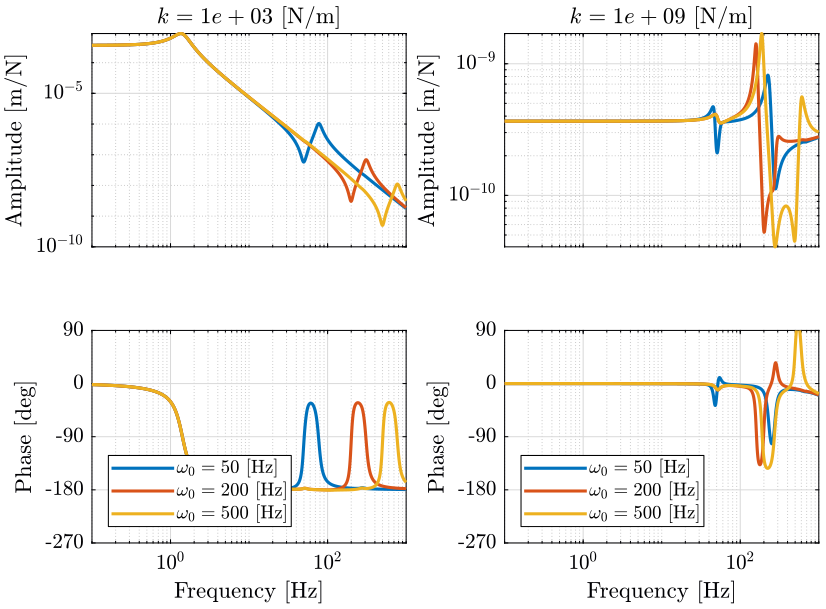
Figure 35: Dynamics from \(\mathcal{F}_z\) to \(\mathcal{X}_z\) for varying payload resonance frequency, both for a soft nano-hexapod and a stiff nano-hexapod
The dynamics for all the payloads (mass from 1kg to 50kg and first resonance from 50Hz to 500Hz) and all the considered nano-hexapod stiffnesses are display in Figure 36.
For nano-hexapod stiffnesses below \(10^6\,[N/m]\):
- the phase stays between 0 and -180deg which is a very nice property for control
- the dynamical change up until the resonance of the payload can be considered as a change of gain
For nano-hexapod stiffnesses above \(10^7\,[N/m]\):
- the dynamics is unchanged until the first resonance which is around 25Hz-35Hz
- above that frequency, the change of dynamics is quite chaotic (which this is due to the micro-station dynamics as shown in the next section) and it would be difficult to have a controller with high bandwidth which is robust to such change of dynamics
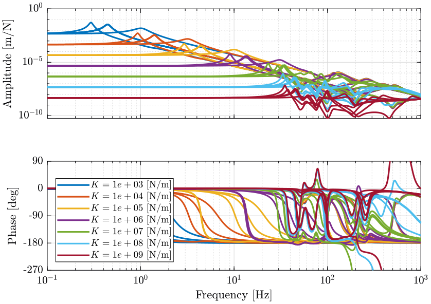
Figure 36: Dynamics from \(\mathcal{F}_z\) to \(\mathcal{X}_z\) for varying payload dynamics, both for a soft nano-hexapod and a stiff nano-hexapod
For soft nano-hexapods, the payload has an important impact on the dynamics that will have to be carefully taken into account for the controller design.
For stiff nano-hexapod, the dynamics doe not change with the payload until the first resonance frequency of the nano-hexapod or of the payload.
If possible, the first resonance frequency of the payload should be maximized (stiff fixation).
Heavy samples with low first resonance mode will be the most problematic.
Effect of Micro-Station Compliance
The micro-station dynamics is quite complex as was shown in Section 2, moreover, its dynamics can change due to:
- a change in some mechanical elements
- a change in the position of one stage. For instance, a large displacement of the micro-hexapod can change the micro-station compliance
- a change in a control loop of some of its stage
Thus, it would be much more robust if the plant dynamics were not depending on the micro-station dynamics. This as several other advantages:
- the control could be develop on top on another support and then added to the micro-station without changing the controller
- the nano-hexapod could be use on top of any other station much more easily
To identify the effect of the micro-station compliance on the system dynamics, the plant dynamics is identified in two different cases (Figure 37):
- with a micro-station considered as a solid body (solid curves)
- with the micro-station dynamics (dashed curves)
One can see that for nano-hexapod stiffnesses below \(10^6\,[N/m]\), the plant dynamics does not significantly changed due to the micro station dynamics (the solid and dashed curves are superimposed).
For nano-hexapod stiffnesses above \(10^7\,[N/m]\), the micro-station compliance appears in the plant dynamics starting at about 45Hz.
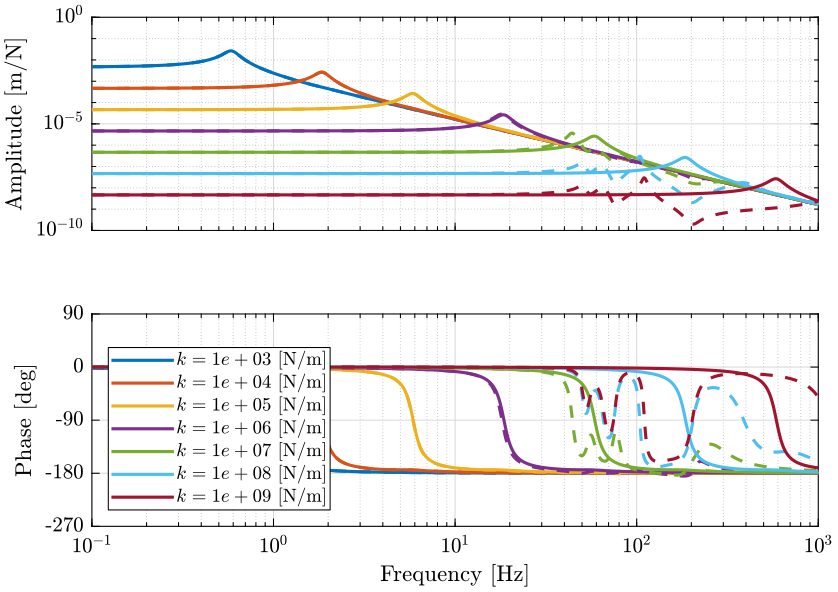
Figure 37: Change of dynamics from force \(\mathcal{F}_x\) to displacement \(\mathcal{X}_x\) due to the micro-station compliance
If the resonance of the nano-hexapod is below the first resonance of the micro-station, then the micro-station dynamics if “filtered out” and does not appears in the dynamics to be controlled. This renders the system robust to any possible change of the micro-station dynamics.
If a stiff nano-hexapod is used, the control bandwidth should probably be limited to around the first micro-station’s mode (\(\approx 45\,[Hz]\)) which will likely no give acceptable performance.
Effect of Spindle Rotating Speed
Let’s now consider the rotation of the Spindle.
The plant dynamics for spindle rotation speed varying from 0rpm up to 60rpm are identified and shown in Figure 38.
One can see that for nano-hexapods with a stiffness above \(10^5\,[N/m]\), the dynamics is mostly not changing with the spindle’s rotating speed.
For very soft nano-hexapods, the main resonance is split into two resonances and one anti-resonance that are all moving at a function of the rotating speed.
The change of dynamics is due to both centrifugal forces and Coriolis forces. This effect has been studied in details in this document.
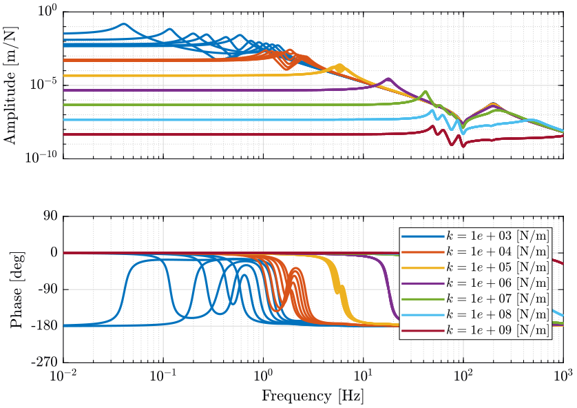
Figure 38: Change of dynamics from force \(\mathcal{F}_x\) to displacement \(\mathcal{X}_x\) for a spindle rotation speed from 0rpm to 60rpm
If the resonance of the nano-hexapod is (say a factor 5) above the maximum rotation speed, then the plant dynamics will be mostly not impacted by the rotation.
A very soft (\(k < 10^4\,[N/m]\)) nano-hexapod should not be used due to the effect of the spindle’s rotation.
Total Plant Uncertainty
Finally, let’s combined all the uncertainties and display the “spread” of the plant dynamics for all the nano-hexapod stiffnesses (Figure 39). This show how the dynamics evolves with the stiffness and how different effects enters the plant dynamics.
Figure 39: Variability of the dynamics from \(\bm{\mathcal{F}}_x\) to \(\bm{\mathcal{X}}_x\) with varying nano-hexapod stiffness
Conclusion
Let’s summarize the findings about the effect of the nano-hexapod’s stiffness on the plant uncertainty:
- The payload’s mass influence the plant dynamics above the first resonance of the nano-hexapod. Thus a high nano-hexapod stiffness helps reducing the effect of a change of the payload’s mass
- The payload’s first resonance is seen as an anti-resonance in the plant dynamics. As this effect will largely be variable from one payload to the other, thus the payload’s first resonance should be maximized (above 300Hz if possible) for all used payloads
- The dynamics of the nano-hexapod is not affected by the micro-station dynamics (compliance) if \(k < 10^6\,[N/m]\)
- The spindle’s rotating speed has no significant influence on the plant dynamics for nano-hexapod’s stiffnesses \(k > 10^5\,[N/m]\)
The resonance frequency of the nano-hexapod should be between 5Hz (way above the maximum rotating speed) and 50Hz (before the first micro-station resonance) for all the considered payloads. This corresponds to an optimal nano-hexapod leg stiffness in the range \(10^5 - 10^6\,[N/m]\).
5.4 Optimal Nano-Hexapod Geometry
Stewart platforms can be studied with:
- Kinematic analysis: study of the geometry of motion without considering the forces and torques that cause the motion
- Jacobian analysis: reveals the relation between the actuators velocities and the moving platform linear and angular velocities. It also constructs the transformation between actuator forces and task space forces
and moments acting on the moving platform.
- Dynamic analysis: consists of the equations of motion for the manipulator which are quite complex to derive
Kinematic and Jacobian analysis are briefly introduced in this section, however the dynamic analysis is not performed analytically but rather studied using the Simscape model.
As will be shown, the Nano-Hexapod geometry has an influence on:
- the stiffness and compliance properties
- the mobility
- the force authority
- the dynamics of the manipulator
Kinematic Analysis
The Kinematic analysis of the Stewart platform can be divided into two problems: the inverse kinematics and the forward kinematics.
For inverse kinematic analysis, it is assumed that the position \({}^A\bm{P}\) and orientation of the moving platform \({}^A\bm{R}_B\) are given and the problem is to obtain the joint variables \(\bm{\mathcal{L}} = \left[ l_1, l_2, l_3, l_4, l_5, l_6 \right]^T\).
This problem can be easily solved, and the obtain joint variables are:
\begin{equation*} \begin{aligned} l_i = &\Big[ {}^A\bm{P}^T {}^A\bm{P} + {}^B\bm{b}_i^T {}^B\bm{b}_i + {}^A\bm{a}_i^T {}^A\bm{a}_i - 2 {}^A\bm{P}^T {}^A\bm{a}_i + \dots\\ &2 {}^A\bm{P}^T \left[{}^A\bm{R}_B {}^B\bm{b}_i\right] - 2 \left[{}^A\bm{R}_B {}^B\bm{b}_i\right]^T {}^A\bm{a}_i \Big]^{1/2} \end{aligned} \end{equation*}If the position and orientation of the platform lie in the feasible workspace, the solution is unique. Otherwise, the solution gives complex numbers.
This means that from the wanted position of the nano-hexapod’s mobile platform with respect to the fixed platform (described by \({}^A\bm{P}\) and \({}^A\bm{R}_B\)) and for a specific geometry (position of the top joints \(^{B}\bm{b}\) and bottom joints \({}^A\bm{a}\)), the required motion of each leg can easily be determined.
In forward kinematic analysis, it is assumed that the vector of limb lengths \(\bm{L}\) is given and the problem is to find the position \({}^A\bm{P}\) and the orientation \({}^A\bm{R}_B\).
This is a difficult problem that requires to solve nonlinear equations.
However, as will be shown in the next section, approximate solution of the forward kinematic analysis can be obtained thanks to the Jacobian analysis.
Jacobian Analysis
The Jacobian matrix \(\bm{J}\) can be computed form the orientation of the legs (describes by the unit vectors \({}^A\hat{\bm{s}}_i\)) and the position of the top joints (described by the position vectors \({}^A\bm{b}_i\)) both expressed in the frame \(\{A\}\):
\begin{equation} \bm{J} = \begin{bmatrix} {\hat{\bm{s}}_1}^T & (\bm{b}_1 \times \hat{\bm{s}}_1)^T \\ {\hat{\bm{s}}_2}^T & (\bm{b}_2 \times \hat{\bm{s}}_2)^T \\ {\hat{\bm{s}}_3}^T & (\bm{b}_3 \times \hat{\bm{s}}_3)^T \\ {\hat{\bm{s}}_4}^T & (\bm{b}_4 \times \hat{\bm{s}}_4)^T \\ {\hat{\bm{s}}_5}^T & (\bm{b}_5 \times \hat{\bm{s}}_5)^T \\ {\hat{\bm{s}}_6}^T & (\bm{b}_6 \times \hat{\bm{s}}_6)^T \end{bmatrix} \end{equation}It can be shown that the Jacobian matrix reveals the relation between the legs’ velocities to the moving platform linear and angular velocities:
\begin{equation} \dot{\bm{\mathcal{L}}} = \bm{J} \dot{\bm{\mathcal{X}}} \label{eq:jacobian_velocity} \end{equation}with:
- \(\dot{\bm{\mathcal{L}}} = [ \dot{l}_1, \dot{l}_2, \dot{l}_3, \dot{l}_4, \dot{l}_5, \dot{l}_6 ]^T\): relative velocity of each strut
- \(\dot{\bm{X}} = [^A\bm{v}_p, {}^A\bm{\omega}]^T\): output twist vector of the mobile platform
For small legs motions \(\delta\bm{\mathcal{L}}\) and small mobile platform motion \(\delta \bm{\mathcal{X}}\), the following approximation can be computed from Eq. \eqref{eq:jacobian_velocity}:
\begin{equation} \delta\bm{\mathcal{L}} \approx \bm{J} \delta\bm{\mathcal{X}}, \quad \delta\bm{\mathcal{X}} \approx \bm{J}^{-1} \delta\bm{\mathcal{L}} \label{eq:jacobian_L} \end{equation}Equations \eqref{eq:jacobian_L} can be used to approximate the forward and inverse kinematic problems for small displacements.
This approximation will be used to estimate the platform’s mobility from the legs’ stroke, or inversely, to estimate the required stroke of the legs from the wanted platform’s mobility.
Note that Eq. \eqref{eq:jacobian_L} is an approximation and is only valid for leg’s displacement less than \(1\%\) of the leg’s length which is the case for the nano-hexapod.
It can also be shown that the Jacobian matrix links the actuator forces to forces and moments acting on the moving platform:
\begin{equation} \bm{\mathcal{F}} = \bm{J}^T \bm{\tau}, \quad \bm{\tau} = \bm{J}^{-T} \bm{\mathcal{F}} \label{eq:jacobian_F} \end{equation}with:
- \(\bm{\tau} = [\tau_1, \tau_2, \cdots, \tau_6]^T\): vector of actuator forces applied in each strut
- \(\bm{\mathcal{F}} = [\bm{f}, \bm{n}]^T\): external force/torque action on the mobile platform
And thus the Jacobian matrix can be used to compute the forces that should be applied by the Stewart platform’s legs from the wanted total forces/torques that is to be applied to the sample.
Linear transformations in Eq. \eqref{eq:jacobian_L} and \eqref{eq:jacobian_F} will be widely in the developed control architectures in Section 6.
Mobility of the Stewart Platform
For a specified geometry and actuator stroke, the mobility of the Stewart platform can be estimated thanks to the approximate forward kinematic analysis.
An example of the mobility considering only pure translations is shown in Figure 40.
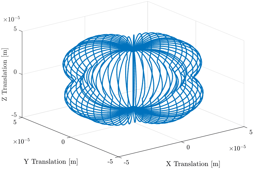
Figure 40: Obtained mobility of a Stewart platform for pure translations (the platform’s orientation is fixed)
From a wanted mobility and a specific geometry, the required actuator stroke can be estimated.
Suppose the following specifications on the mobility:
- x, y and z translations up to \(50\,\mu m\)
- x and y rotation up to \(30\,\mu rad\)
- no z rotation
The geometry is chosen arbitrary and corresponds to the wanted nano-hexapod size.
If only pure translations and pure rotations are considered, the required actuator stroke is \(76 \mu m\), whereas if combined translations and rotations are considered, the required actuator stroke is \(177 \mu m\).
This gives an idea of the relation between the mobility and the actuator stroke.
Stiffness and Compliance matrices
In order to determine the stiffness and compliance matrices of the Stewart platform, let’s model the actuators by a spring with a stiffness \(k_i\) in parallel with a force source \(\tau_i\).
The stiffness of the actuator \(k_i\) links the applied (constant) actuator force \(\delta \tau_i\) and the corresponding small deflection \(\delta l_i\):
\begin{equation*} \tau_i = k_i \delta l_i, \quad i = 1,\ \dots,\ 6 \end{equation*}Combining these 6 relations:
\begin{equation*} \bm{\tau} = \mathcal{K} \delta \bm{\mathcal{L}} \quad \mathcal{K} = \text{diag}\left[ k_1,\ \dots,\ k_6 \right] \end{equation*}Equations \eqref{eq:jacobian_L} and \eqref{eq:jacobian_F} are used to obtain:
\begin{equation} \bm{\mathcal{F}} = \bm{K} \delta \bm{\mathcal{X}} \end{equation}with the stiffness matrix
\begin{equation} \bm{K} = \bm{J}^T \mathcal{K} \bm{J} \label{eq:jacobian_K} \end{equation}And the compliance matrix can be computed by taking the inverse of the Stiffness matrix:
\begin{equation*} \bm{C} = \bm{K}^{-1} = (\bm{J}^T \mathcal{K} \bm{J})^{-1} \end{equation*}The compliance matrix of a manipulator shows the mapping of the moving platform wrench applied at \(\bm{O}_B\) to its small deflection by
\begin{equation*} \delta \bm{\mathcal{X}} = \bm{C} \cdot \bm{\mathcal{F}} \end{equation*}Stiffness properties of the Stewart platform can then be estimated from the architecture (through the Jacobian matrix) and leg’s stiffness.
Effect of a change of geometry
Equations \eqref{eq:jacobian_L}, \eqref{eq:jacobian_F} and \eqref{eq:jacobian_K} can be used to see how the maneuverability, the force authority and the stiffness of the Stewart platform are changing with a the geometry (position of the joints and orientation of the legs).
The effects of two changes in the manipulator’s geometry, namely the position and orientation of the legs, are summarized in Table 1. These results could have been easily deduced based on some mechanical principles, but thanks to the kinematic analysis, they can be quantified.
| legs pointing more vertically | legs further apart | |
|---|---|---|
| Vertical stiffness | \(\nearrow\) | \(=\) |
| Horizontal stiffness | \(\searrow\) | \(=\) |
| Vertical rotation stiffness | \(\searrow\) | \(\nearrow\) |
| Horizontal rotation stiffness | \(\nearrow\) | \(\nearrow\) |
| Vertical force authority | \(\nearrow\) | \(=\) |
| Horizontal force authority | \(\searrow\) | \(=\) |
| Vertical torque authority | \(\searrow\) | \(\nearrow\) |
| Horizontal torque authority | \(\nearrow\) | \(\nearrow\) |
| Vertical stroke | \(\searrow\) | \(=\) |
| Horizontal stroke | \(\nearrow\) | \(=\) |
| Vertical rotation stroke | \(\nearrow\) | \(\searrow\) |
| Horizontal rotation stroke | \(\searrow\) | \(\searrow\) |
Even tough Table 1 can be used to optimize the nano-hexapod’s geometry, the available space for the nano-hexapod is too small to obtain a significant impact on the manipulator’s stiffness and stroke.
Cubic Architecture
A very popular choice of Stewart platform architecture in the scientific literature, especially for vibration isolation, is the Cubic architecture.
The cubic architecture is quite specific in the sense that the active struts are arranged in a mutually orthogonal configuration connecting the corners of a cube (Figure 41).
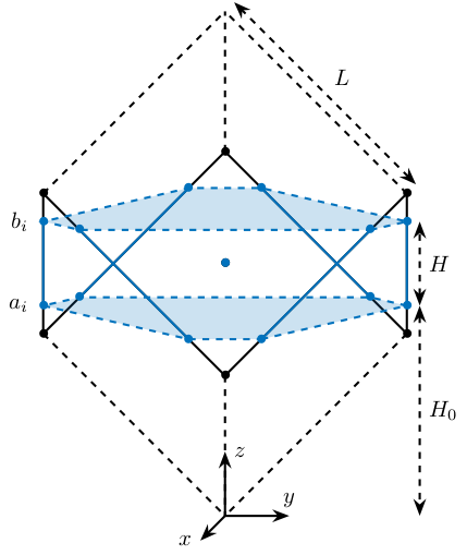
Figure 41: Schematic representation of the Cubic architecture
This architecture provides some advantages such as uniform stiffness and uniform mobility in all directions. It can also have very nice dynamical properties in specific conditions (center of mass of the payload located at the cube’s center) that are not met for the NASS.
The cubic configuration also puts much restriction on the position and orientation of the legs as there is only one design variable: the size of the cube.
For these reasons, the cubic configuration is not recommended for the nano-hexapod.
[5] and [6] are good resources about the Cubic architecture for vibration isolation. Separate study of the cubic architecture is performed here.
Effect of Flexible Joints
Each of the nano-hexapod legs has a universal joint at one end and a spherical joint at the other end.
When only small stroke is required, flexible joints can be used: material is bend to achieve motion, rather than relying on sliding or rolling across two surfaces.
Example of flexible joints used for Stewart platforms are shown in Figures 42 and 43.
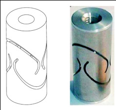
Figure 42: Flexible joints used in preumont07_six_axis_singl_stage_activ
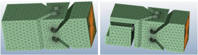
Figure 43: An alternative type of flexible joints that has been used for Stewart platforms yang19_dynam_model_decoup_contr_flexib
The flexible joints have few advantages compared to conventional joints such as the absence of wear, friction and backlash which allows extremely high-precision (predictable) motion.
The parasitic bending and torsional stiffness of these joints usually induce some limitation on the control performance.
This has been studied using the Simscape model (report available here), and conclusions on the required characteristics of the flexible joints are summarized below.
The bending and torsional stiffnesses somehow adds a parasitic stiffness in parallel with the struts. This is not found to be problematic for the control architecture that will be developed in Section 6 (it is however, if Integral Force Feedback is to be used, explained here).
The finite axial stiffness of the flexible joints can however be very problematic for control. Small values of the axial stiffness are shown to limit the achievable damping using Direct Velocity Feedback. The axial stiffness should therefore be maximized and taken into account in the model of the nano-hexapod.
For the identified optimal actuator stiffness \(k = 10^5\,[N/m]\), the flexible joint should have the following stiffness properties:
- Axial Stiffness: \(K_a > 10^7\,[N/m]\)
- Bending Stiffness: \(K_b < 50\,[Nm/rad]\)
- Torsion Stiffness: \(K_t < 50\,[Nm/rad]\)
These requirements are easily obtained in practice. For instance, the flexible joint used for the ID16 nano-hexapod have the following stiffness properties:
- Axial Stiffness: \(K_a = 6 \cdot 10^7\,[N/m]\)
- Bending Stiffness: \(K_b = 15\,[Nm/rad]\)
- Torsion Stiffness: \(K_t = 20\,[Nm/rad]\)
Even though much attention should be paid on the proper design of the flexible joints, they should not impose limitation on the performance of the system.
Simulations will help determine the required rotational stroke of the flexible joints and will help with the design.
Conclusion
Relations between the geometry of the Stewart platform and its characteristics such as stiffness, maneuverability and force authority have been derived.
These relations can help optimize the Stewart platform’s geometry, however, the choice of the geometry is quite constrained by the limited size of the hexapod, the size of the flexible joints and of the included actuators and sensors.
The effects of flexible joints stiffness on the dynamics have been studied and requirements on the flexible joints have been derived.
5.5 Flexible Elements
The multi-body model of the micro-station as well as of the nano-hexapod are composed of solid bodies connected with springs and dampers.
This is valid for the micro-station are shown by the measurements in Section 2 but this may not be the case for the nano-hexapod.
In order to take into account the flexibility of some of the nano-hexapod mechanical parts, some tools have been developed to integrate flexible elements into a Simscape model.
The procedure is as follow:
- import the geometry into Ansys
- mesh the element and select the nodes of interest (interface with other elements, points where forces should be applied or displacement measure)
- select the number of modes to take into account
- apply a Guyan Reduction that computes the reduced mass and stiffness matrices
- import into Matlab the mass matrix, stiffness matrix as well as the coordinates of the interface nodes
- import the matrices into Simscape. The flexible element can then be interfaced with other simscape elements
Mainly two elements will be modeled using this technique: the flexible joints and the amplified piezoelectric actuators.
More detailed information about the modelling technique is available here.
5.5.1 Flexible Piezoelectric actuators
In order to test this modeling technique, some tests have been performed on a flexible piezoelectric stack actuator.
The APA95ML from Cedrat has been sketched into Ansys and the interface nodes chosen as shown in Figure 44. The top and bottom nodes are used as interface nodes to connect to other mechanical parts of the nano-hexapod. The ten interface nodes along the piezo stack are used to apply forces into the stack.
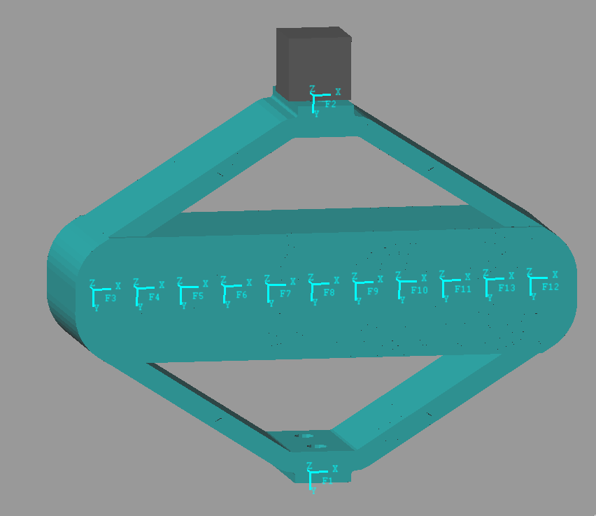
Figure 44: Geometry of the amplified piezoelectric actuator (APA95ML) as well as the chosen interface nodes
The reduced mass and stiffness matrices are exported using Ansys and imported into Matlab. The actuator is included in a Simscape model, and the dynamics from forces applied by the piezo stack to the vertical displacement of the amplified structure is identified using Simscape and compare with an harmonic response using Ansys (Figure 45).
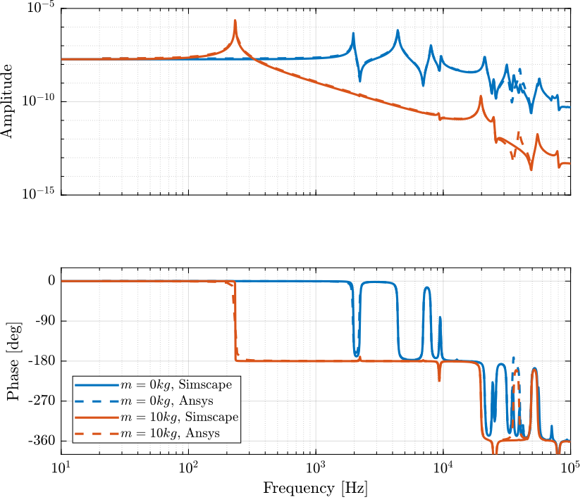
Figure 45: Comparison of the obtained dynamics using Simscape with the harmonic response analysis using Ansys
A payload with a mass of 10kg is then added both in the Simscape model and in Ansys and the dynamic is identified again and compared (Figure 45). The dynamics obtained with Simscape and Ansys are very close to each other which validate the fact that we can interface the flexible element with other Simscape parts.
5.5.2 Test Bench
A test bench is planned to validate the presented modelling technique.
The DCM’s fast jack test bench will be slightly modified to integrate the APA95ML actuator (already available).
The idea is to identify the transfer functions from forces applied by the stack actuator to the vertical displacement as what done both using Simscape and Ansys.
This test bench requires very little work and will permit to gain much confident on the modelling technique used as well as on the dynamics of amplified piezoelectric actuators.
5.5.3 Design Methodology
During all the mechanical design of the nano-hexapod, it is planned to use the presented modelling technique to ensure that no parasitic modes will be problematic for the control part.
More specifically, it is wanted that both the flexible joints and the amplified piezoelectric actuators do not introduce parasitic modes in the dynamics to be controlled up to 200Hz.
This flexible modeling technique is thus a very important element during the mechanical design of the nano-hexapod.
5.6 Conclusion
In Section 5.2, it has been concluded that a nano-hexapod stiffness below \(10^5-10^6\,[N/m]\) helps reducing the high frequency vibrations induced by all sources of disturbances considered. As the high frequency vibrations are the most difficult to compensate for when using feedback control, a soft hexapod will most certainly helps improving the performances.
In Section 5.3, it has been concluded that a nano-hexapod leg stiffness in the range \(10^5 - 10^6\,[N/m]\) is a good compromise between the uncertainty induced by the micro-station dynamics and by the rotating speed. Provided that the samples used have a first mode that is sufficiently high in frequency, the total plant dynamic uncertainty should be manageable by the control.
Thus, a leg’s stiffness of \(10^5\,[N/m]\) will be used in Section 6 to develop the robust control architecture and to perform simulations.
A more detailed study of the determination of the optimal stiffness based on all the effects is available here.
Finally, in section 5.4 some insights on the wanted nano-hexapod geometry are given.
6 Robust Control Architecture
Before designing the control system, let’s summarize what have been done:
- The multi-body model of the micro-station has been tuned based on actual dynamical measurements
- Ground motion and stage vibrations have been estimated and included in the model
- The optimal nano-hexapod stiffness has been determined such that it minimizes the effect of disturbances and at the same time reduces the plant dynamic uncertainty
The optimal nano-hexapod is now included in the model, and a robust control architecture is developed.
Note that it is preferred to design one controller that gives acceptable performance for all the changes in the system (payload masses, spindle’s rotation speeds, etc). This control property is referred to as robust performance. This is however quite challenging as the plant dynamics changes a lot with experimental conditions such as a change of payload’s mass.
If it turns out that no robust controller can give acceptable performance, an alternative would be to develop an adaptive controller that depends on the payload mass/inertia. This would however require to measure the mass/inertia of each used payload and to manually choose the controller that was designed for that particular mass/inertia.
This part is divided in the following sections:
- Section 6.1: the High Authority Control / Low Authority Control Architecture is described and the reasons of its use are explained
- Section 6.2: the active damping strategy is implemented and its effects on the system are described
- Section 6.3: the high authority control is developed and the control robustness is studied
- Section 6.4: tomography experiments are simulated and the performances are estimated
- Section 6.5: more complex simulations are performed to further validate this control architecture
6.1 High Authority Control / Low Authority Control Architecture
There exist many control architectures that could be used on Stewart platforms. One of the them that seems the most adapted for the NASS is called the High Authority Control / Low Authority Control (HAC-LAC) architecture.
Some interesting properties of the HAC-LAC architecture are summarized below (taken from [7]):
The HAC/LAC approach consist of combining the two approached in a dual-loop control as shown in Figure 46. The inner loop uses a set of collocated actuator/sensor pairs for decentralized active damping with guaranteed stability ; the outer loop consists of a non-collocated HAC based on a model of the actively damped structure. This approach has the following advantages:
- The active damping extends outside the bandwidth of the HAC and reduces the settling time of the modes which are outsite the bandwidth
- The active damping makes it easier to gain-stabilize the modes outside the bandwidth of the output loop (improved gain margin)
- The larger damping of the modes within the controller bandwidth makes them more robust to the parmetric uncertainty (improved phase margin)
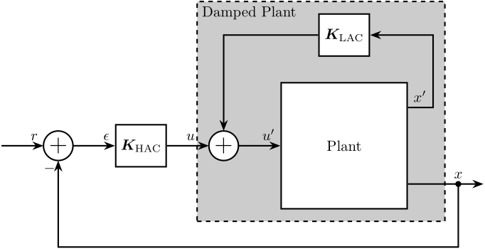
Figure 46: HAC-LAC Architecture with a system having only one input
The HAC-LAC architecture thus consists of two cascade controllers:
6.2 Active Damping and Sensors to be included in the nano-hexapod
Three active damping techniques could be applied for the Low Authority Control:
- Integral Force Feedback
- Direct Velocity Feedback with relative motion sensors
- Direct Velocity Feedback with inertial sensors
To determine the most suited active damping technique, they are compared based on their ability to (reports accessible here and here):
- reduce the effect of disturbances
- render the plant dynamics simpler to control for the High Authority Controller
- remains stable for all changes in the system
The conclusions are (summarized in Table 2):
- Integral Force Feedback is to be avoided as it renders the system unstable when the nano-hexapod’s is rotating (effect explained in the next section)
- Direct velocity feedback with inertial sensor should also be avoided as it would tends to decouple the motion of the sample from the motion of the granite (which is not wanted). It also does not give the wanted robustness properties
- Direct velocity feedback with relative motion sensors can be used to damp the nano-hexapod’s modes in a robust way. It however may increases the sensibility to stages vibrations at higher frequency
| Integral Force Feedback | Direct Velocity Feedback | Inertial Control | |
|---|---|---|---|
| Sensors to be included | Force Sensors | Relative Motion Sensors | Inertial Sensors |
| Advantages | Low noise | Guaranteed Stability | Increase the compliance and reduces the transmissibility |
| Easy integration with piezoelectric actuators | Arbitrary damping added to the nano-hexapod | ||
| Disadvantages | Reduces the compliance at low frequency | Increases the transmissibility at high frequency | No guaranteed stability |
| No guaranteed stability in presence of rotation | Increases the sensibility to ground motion |
Relative Direct Velocity Feedback is found to be the most suitable active damping techniques for the nano-hexapod. Therefore, relative motion sensors must be integrated in the six nano-hexapod’s legs.
Effect of the Spindle’s Rotation - Guaranteed Stability
To see why Integral Force Feedback should not be applied to damp the nano-hexapod’s modes, a simple model of a rotating positioning platform integration force sensors has been developed (described in details here).
The platform main resonance frequency is \(\omega_0\) and the rotation speed is \(\omega\).
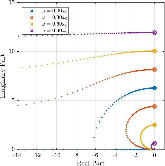
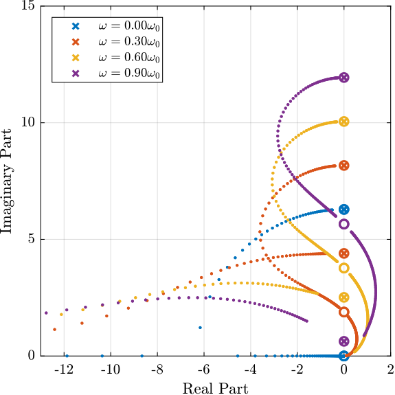
Root Locus plots for Integral Force Feedback and Direct Velocity Feedback are shown in Figure 3. These plots show the evolution of the system’s poles in the complex plane as a function of the control gain.
 |
 |
| Direct Velocity Feedback | Integral Force Feedback |
To understand what the root locus means, consider Figure 47 where two resonant systems are compared:
- The first one (represented in blue) is undamped. The corresponding poles of this system is located on the imaginary axis.
- The second one (represented in red) has some added damping which can be easily see by the reduction of the amplitude near the resonance. On the complex plane, this is manifested by the being “moved” such that the angle \(\phi\) it makes with the imaginary axis is increase.
As a matter of fact, the damping ratio of a system resonance can be approximated by \(\xi \approx \sin \phi\).
To damp a system, it is thus wanted to move the poles to the left part of the complex plane. A pole with a positive real part corresponds to an unstable system, and thus the right part of the complex should be avoided.
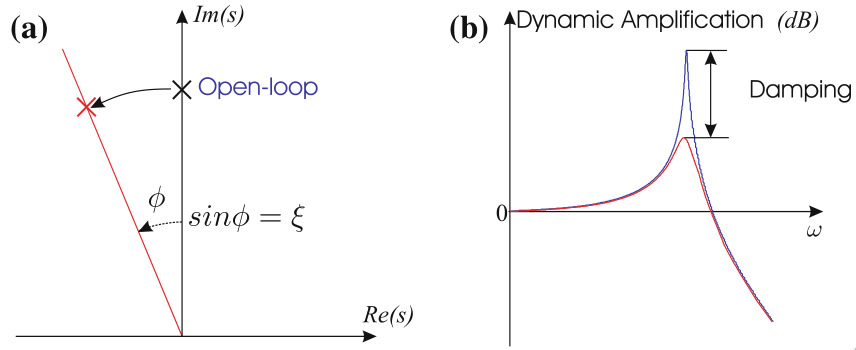
Figure 47: Role of damping (preumont18_vibrat_contr_activ_struc_fourt_edition). (a) Pole position in the complex plane. (b) Change of dynamic amplification (\(1/2\xi\))
Coming back to the Root Locus in Figure 3, it can be seen that:
- For Direct Velocity Feedback:
- The system’s poles are staying in the left half plane which means guaranteed stability
- Arbitrary damping can be added to the system’s resonances
- For Integral Force Feedback:
- For non-null rotation speed, and whatever the control gain is, a pole is located in the right part of the complex plane, showing that the closed-loop system is unstable
- Limited damping can be added to the system
Similar observations are made using the Simscape model of the NASS, and this shows why Direct Velocity Feedback is the most suitable active damping technique for the NASS.
Relative Direct Velocity Feedback Architecture
Relative motion sensors are included in each of the nano-hexapod’s leg and a decentralized direct velocity feedback control architecture is applied (Figure 48).
The signals shown in Figure 48 are:
- \(\bm{\tau}\): Actuator forces applied in each leg
- \(\bm{\tau}_m\): Force sensor signal located in each leg (not used here)
- \(\bm{\mathcal{X}}\): Measurement of the payload position with respect to the granite by the metrology system (used for the HAC part)
- \(d\bm{\mathcal{L}}\): Measurement of the (small) relative motion of each leg
\(\bm{K}_{\text{DVF}}\) is a diagonal controller with derivative action. This control architecture is equivalent as to have six independent control loops from the relative motion sensor of one leg to the actuator of the same leg (hence the term decentralized). The force applied in each leg being proportional to the relative velocity of the associated leg (thanks to the derivative action), this is equivalent as adding damping in each of the legs.
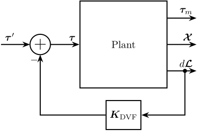
Figure 48: Low Authority Control: Decentralized Direct Velocity Feedback
Dynamics and Root Locus
The dynamics from \(\tau_i\) to \(d\mathcal{L}_i\) for three payload masses is shown in Figure 49. It is shown that for all the payload masses, the dynamics shows an alternation of poles and zeros which makes the direct velocity feedback loop robust.
This is confirmed by the Root Locus in Figure 50 where all the poles are staying in the left half plane. Moreover, it is seen that arbitrary damping can be applied to the nano-hexapod’s modes.
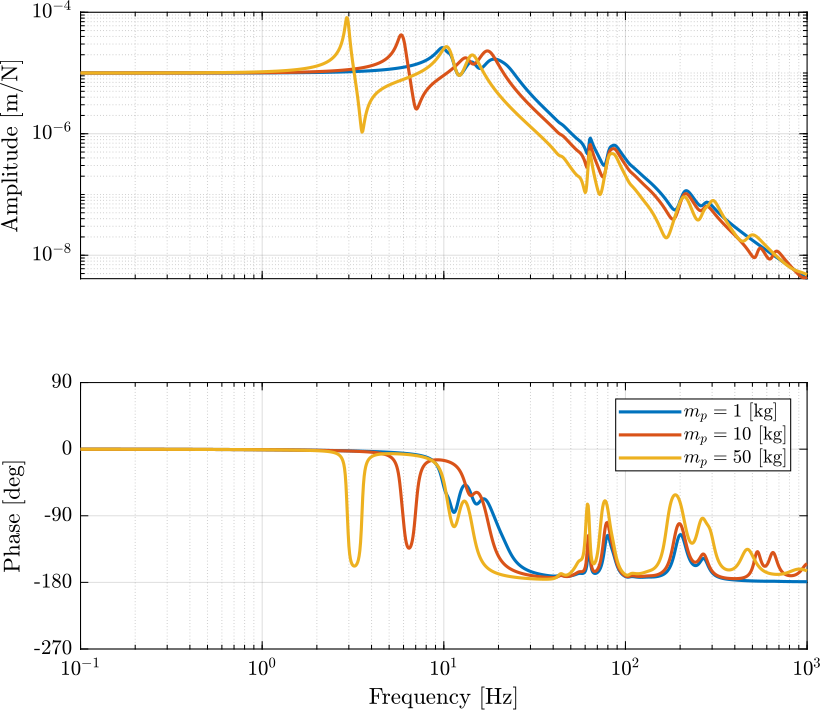
Figure 49: Dynamics from actuator force \(\tau_i\) to the relative displacement of the corresponding leg \(d\mathcal{L}_i\) for three payload masses
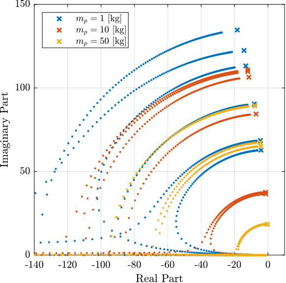
Figure 50: Root Locus (zoomed on the nano-hexapod modes) corresponding to the Direct Velocity Feedback control for three payload masses
The DVF gain is here chosen in such a way that the suspension modes of the nano-hexapod are critically damped whatever the sample mass.
This may not be the optimal choice as will be further explained.
Effect of Active Damping on the Sensibility to Disturbances
One objective of the active damping technique is to lower the sensibility to disturbances which are shown in Figure 51 without active damping (solid) and with the use of DVF (dashed).
The Direct Velocity Feedback control lowers the sensibility to disturbances in the vicinity of the nano-hexapod resonance but increases the sensibility at higher frequencies.
A smaller control gain could probably limit the increase of the sensibility at higher frequencies while still providing sufficient sensibility reduction near the nano-hexapod resonances. Further optimization of the gain should then be performed.
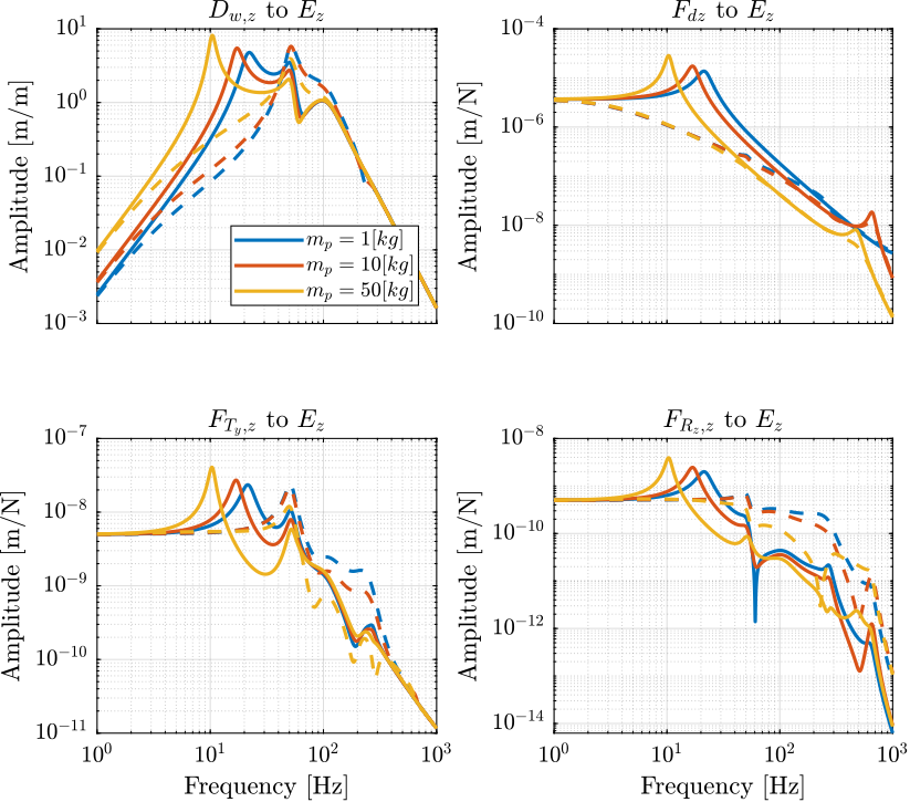
Figure 51: Norm of the transfer function from vertical disturbances to vertical position error with (dashed) and without (solid) Direct Velocity Feedback applied. Disturbances are: ground motion (top left), direct forces (top right), translation stage vibration (bottom left) and spindle vibrations (bottom right)
Effect of Active Damping on the Primary Plant Dynamics
Another control objective for the LAC is to render the plant dynamics simpler to control for the High Authority Controller.
The plant dynamics before (solid curves) and after (dashed curves) the Low Authority Control implementation are compared in Figure 52. It is clear that the use of the DVF reduces the dynamical spread of the plant dynamics between 5Hz and 100Hz. This will make the primary controller more robust and easier to develop.
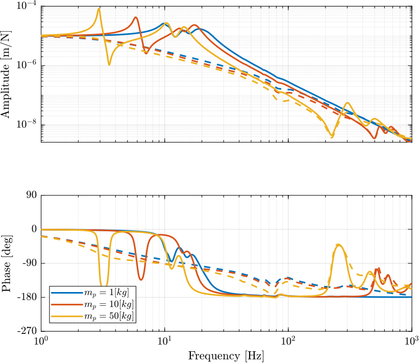
Figure 52: Primary plant in the space of the legs with (dashed) and without (solid) Direct Velocity Feedback
Conclusion
It has been shown that Direct Velocity Feedback using relative motion sensors is the most adapted active damping technique to be applied to the nano-hexapod.
Its main disadvantage is the increase of the sensibility to stage vibrations at high frequency which may limit the performances of the system.
Thus, further improvements and optimization will be applied to this control architecture in order to limit the increase of vibration transmissibility at high frequency.
6.3 High Authority Control
The High Authority Controller objective is to stabilize the position of the sample with respect to the granite.
It might be the most important element of the control architecture as it acts directly based on the actual sample’s position.
Its proper design will most likely determine the performance of the system.
Control in the Task space or in the Leg Space?
Let’s consider the two HAC-LAC control architectures shown in Figures 53 and 54 where an outer control loop is added to the already damped plant.
The control objective for the High Authority Controller \(\bm{K}\) is to compute the force \(\bm{\tau}^\prime\) to be applied by the six nano-hexapod’s actuators such that the relative position of the sample with respect to the granite \(\bm{\mathcal{X}}\) follows a wanted trajectory \(\bm{r}_\mathcal{X}\).
To do so, the block Compute Pos. Error is used to compute the position error \(\bm{\epsilon}_{\mathcal{X}_n}\) of the sample with respect to the nano-hexapod’s base platform from the actual measurement of the sample’s pose \(\bm{\mathcal{X}}\) and the wanted pose \(\bm{r}_\mathcal{X}\).
The computation done in such block was briefly explained in Section 4.3.
The two proposed control architectures are very similar in the sense that their outcome is a multi-input multi-output controller \(\bm{K}\). The difference between the two architectures relies in the way the controllers are designed:
- For the architecture shown in Figure 53:
- The controller \(\bm{K}_\mathcal{X}\) is designed in the task space: from the position/orientation error \(\bm{\epsilon}_{\mathcal{X}_n}\), it generates a force/torque \(\bm{\mathcal{F}}\) to be applied to sample
- The forces/torques are then further converted to actuators forces \(\bm{\tau}^\prime\) with the use of the Jacobian matrix \(\bm{J}^{-T}\)
- The full controller is \(\bm{K} = \bm{J}^{-T} \bm{K}_\mathcal{X}\)
- For the architecture shown in Figure 54:
- The sample’s position error \(\bm{\epsilon}_{\mathcal{X}_n}\) is first converted to the corresponding length errors of the six nano-hexapod’s legs \(\bm{\epsilon}_\mathcal{L}\) with the approximate inverse kinematics using the Jacobian matrix \(\bm{J}\)
- The controller \(\bm{K}_\mathcal{L}\) then computes the actuator forces \(\bm{\tau}^\prime\) such that each of the legs have the wanted displacement
- The full controller is \(\bm{K} = \bm{K}_\mathcal{L} \bm{J}\)

Figure 53: HAC-LAC architecture. The inner loop consist of a decentralized Direct Velocity Feedback. The outer loop consist of position control in the task space
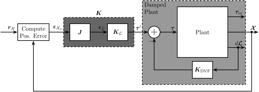
Figure 54: HAC-LAC architecture. The inner loop consist of a decentralized Direct Velocity Feedback. The outer loop consist of position control in the leg’s space
The choice of whether the controller should be designed in the leg space or in the task space does however makes some differences, that can be seen by looking at the dynamics to be controlled:
- Typical dynamics from \(\bm{\mathcal{F}}\) to \(\bm{\epsilon}_{\mathcal{X}_n}\) is shown in Figure 55:
- The suspension modes of the Stewart platform are separated, and the direct (diagonal) dynamical terms are different
- The coupling is very small except for the dynamics from \(\mathcal{F}_{x,y}\) to \(R_{y,x}\) and from \(\mathcal{M}_{x,y}\) to \(D_{y,x}\) which is due to an non-diagonal stiffness and mass matrices
- Typical dynamics from \(\bm{\tau}\) to \(\bm{\epsilon}_\mathcal{L}\) is shown in Figure 56:
- The dynamics from \(\tau_i\) to \(d\mathcal{L}_i\) are all identical and contains all the Stewart platform modes, and thus only one controller has to be designed
- The coupling is small at low frequency, quite high near the suspension modes of the Stewart platform and then small again at high frequency
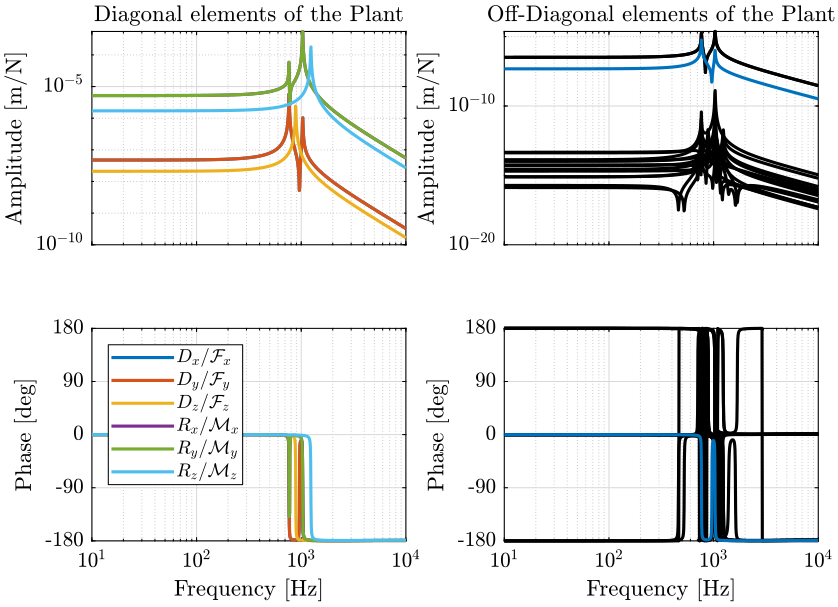
Figure 55: Direct (diagonal) dynamical terms (left) and coupled terms (right, shown in black) for the plant in the task space
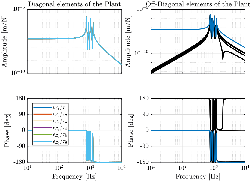
Figure 56: Direct (diagonal) dynamical terms (left) and coupled terms (right, shown in black) for the plant in the leg space
The differences of a control in the leg space and in the task space are summarized in Table 4.
| Control in the leg space | Control in the task space | |
|---|---|---|
| Plant Meaning | \(\delta\mathcal{L}_i/\tau_i\) | \(\delta\mathcal{X}_i/\mathcal{F}_i\) |
| Obtained Decoupling | Decoupled at DC | Dynamical decoupling except few terms |
| Diagonal Elements | Identical with all the Resonances | Different, resonances are cancel out |
| Mechanical Architecture | Architecture Independent | Better with Cubic Architecture |
| Advantages | One controller to be designed | Possible to have different controllers for each |
| direction as the requirements are not the same |
Both control architecture have been applied and the control in the leg space appears to be simpler to apply and have good robustness properties.
An alternative that could increase the control performance and robustness would be to design the full multi-input multi-outputs controller \(\bm{K}\) in one step using optimal and robust control synthesis techniques such as the \(\mathcal{H}_\infty\) loop shaping.
Plant Dynamics in the leg space
The plant dynamics from \(\tau_i\) to \(\epsilon_{\mathcal{L}_i}\) for each of the six legs and for the three payload’s masses is shown in Figure 57. The dynamical spread is kept reasonably small thanks to both the optimal nano-hexapod design and the Low Authority Controller.
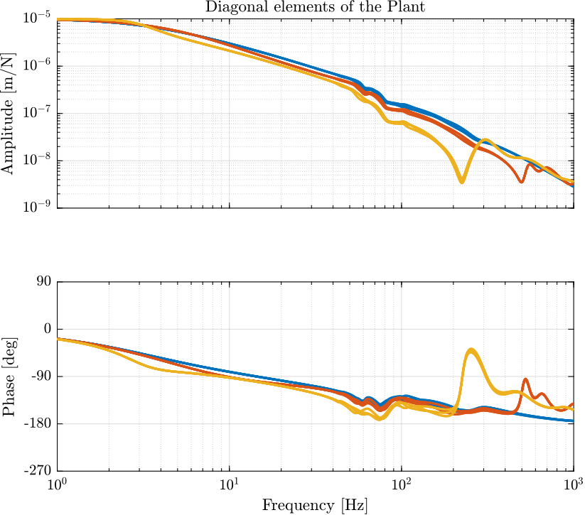
Figure 57: Diagonal elements of the transfer function matrix from \(\bm{\tau}^\prime\) to \(\bm{\epsilon}_{\mathcal{X}_n}\) for the three considered masses
Controller Design
The diagonal controller \(\bm{K}_\mathcal{L}\) is then tuned in such a way that the control bandwidth is around 100Hz and such that enough stability margins are obtained for all the payload’s masses. The obtained loop gain is shown in Figure 58.
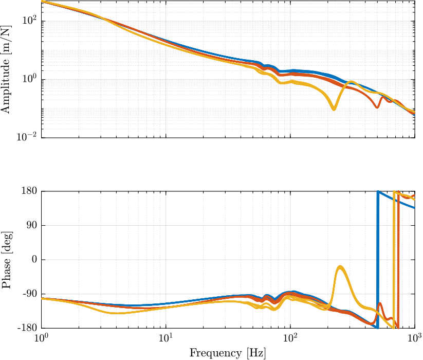
Figure 58: Loop gain for the primary plant
Noise Budgeting
The sensibility to disturbance after the use of HAC-LAC control is shown in Figure 59. The change of sensibility is very typical for feedback system:
- the sensibility is reduced within the controller bandwidth (here \(\approx 100\,[Hz]\))
- the sensibility is increase around the crossover frequency and mostly unchanged outside of the control bandwidth
The large increase at around 250Hz when using a mass of either 1kg or 10kg is probably caused by insufficient stability margins.
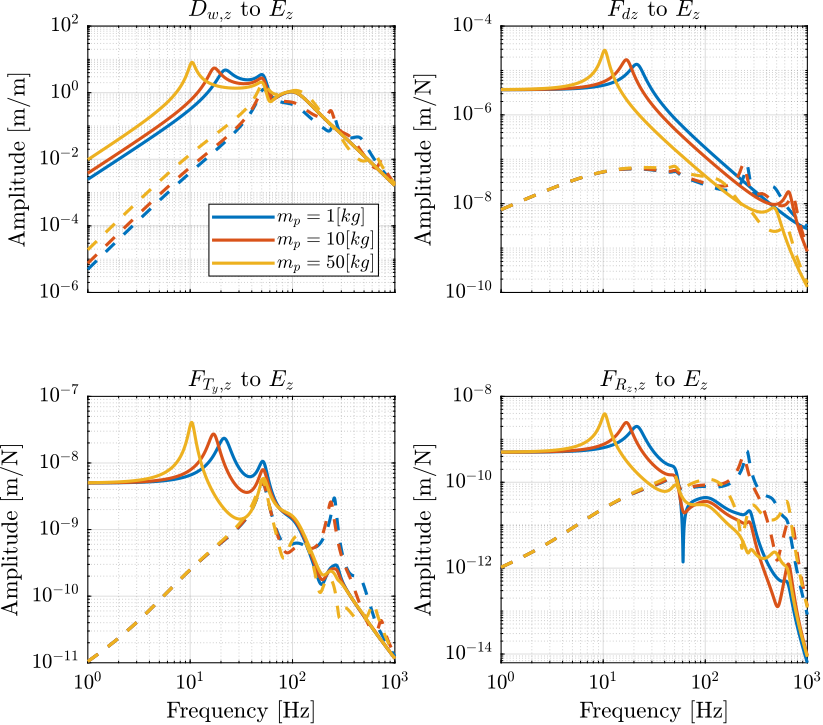
Figure 59: Sensibility to disturbances when the HAC-LAC control is applied (dashed) and when it is not (solid)
6.4 Simulation of Tomography Experiments
Simulation Setup
A simulation of a tomography is performed with the optimal nano-hexapod and the HAC-LAC architecture implemented. The results of this simulation are compared to the simulation performed in Section 4.4 without the nano-hexapod. All the disturbances are included such as ground motion, spindle and translation stage vibrations.
Frequency Analysis
The Power Spectral Density of the sample’s position error is plotted in Figure 60 and the Cumulative Amplitude Spectrum is shown in Figure 61. The top three plots corresponds to the X, Y and Z translations and the bottom three plots corresponds to the X,Y and Z rotations.
Several observations can be made:
- The sample’s vibrations are reduced within the control bandwidth as was expected
- The obtained performances for all the three considered masses are very similar. This is an indication of the good system’s robustness
- From the Cumulative Amplitude Spectrum (Figure 61), it can be seen that Z motion is reduced down to \(\approx 30\,nm\,[rms]\) and the Y motion down to \(\approx 25\,nm\,[rms]\)
An increase in the rotational vibrations is observed. This is due to the fact that:
- no perturbations inducing rotations were included in the simulation and thus the rotational vibrations are very small
- the high authority control induces some coupling between translations and rotations. It then introduces some rotational motion due to vibrations in translation
This increase in rotation is still very small and is not foreseen to be a problem
- The vertical rotation plot is meaningless as the spindle rotation was considered to be perfect and no attempt was made to compensate these vibrations by the nano-hexapod
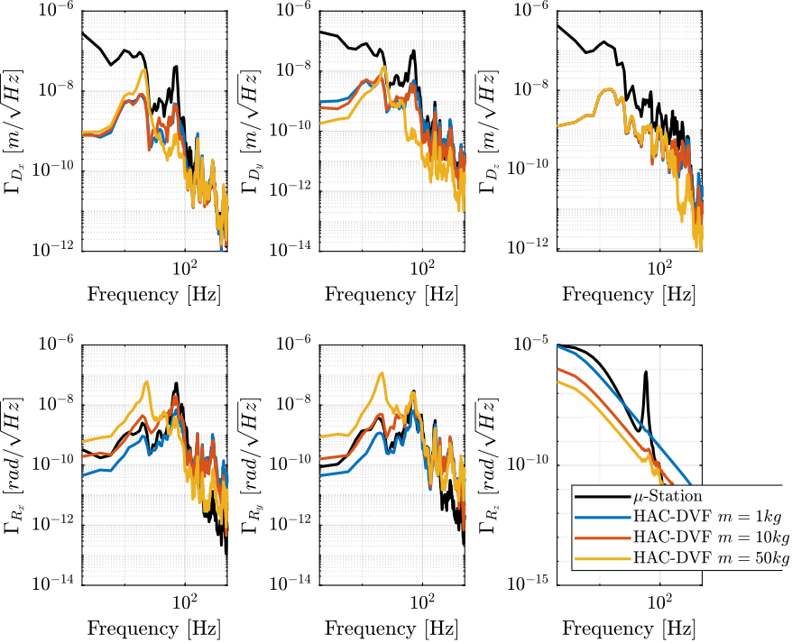
Figure 60: Amplitude Spectral Density of the position error in Open Loop (black) and with the HAC-LAC controller for three payload masses
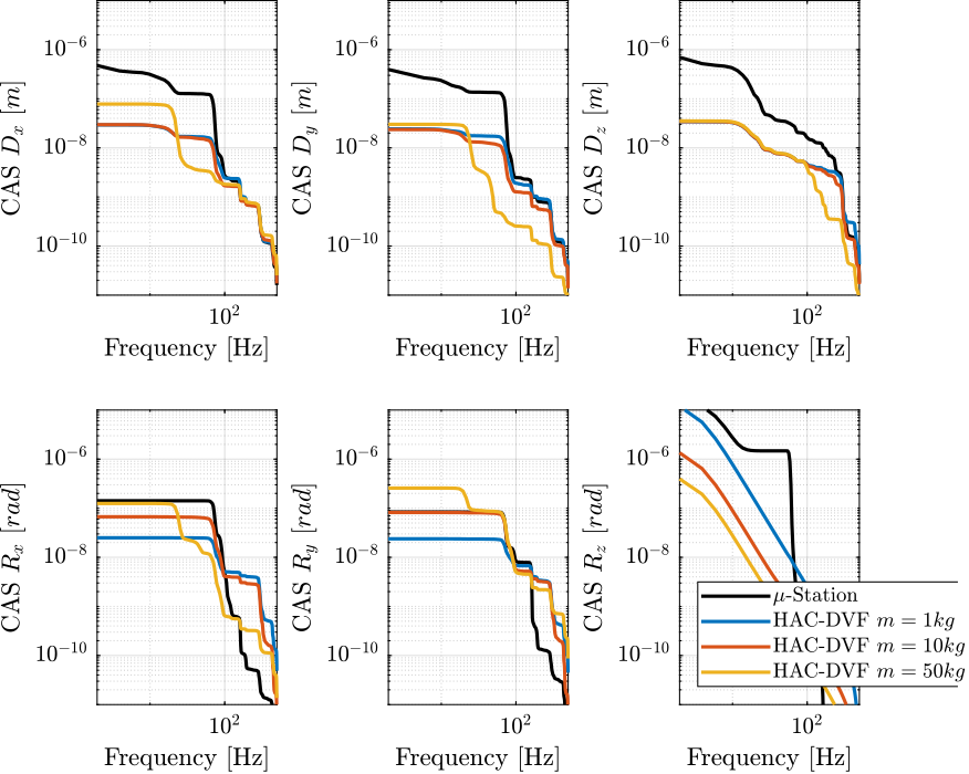
Figure 61: Cumulative Amplitude Spectrum \(CAS_{-}\) of the position error in Open Loop (black) and with the HAC-LAC controller for three payload masses
Time Domain Analysis
The time domain sample’s vibrations are shown in Figure 62. The use of the nano-hexapod combined with the HAC-LAC architecture is shown to considerably reduce the sample’s vibrations.
An animation of the experiment is shown in Figure 63 and it can be seen that the actual sample’s position is more closely following the ideal position compared to the simulation of the micro-station alone in Figure 26 (same scale was used for both animations).
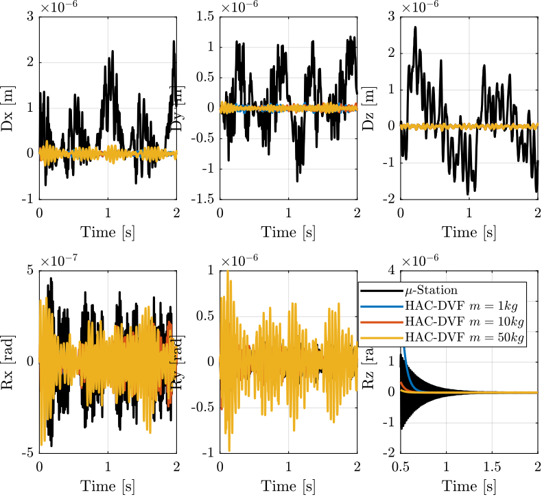
Figure 62: Position Error of the sample during a tomography experiment when no control is applied and with the HAC-DVF control architecture

Figure 63: Tomography Experiment using the Simscape Model in Closed Loop with the HAC-LAC Control - Zoom on the sample’s position (the full vertical scale is \(\approx 10 \mu m\))
6.5 Simulation of More Complex Experiments
Two additional simulations of experiments are performed:
- A tomography experiment with a micro-hexapod’s motion to align a particular location of the sample with the X-ray. The center of mass of the sample is then no longer aligned with the spindle’s rotation axis.
- A simultaneous spindle’s rotation and scans using the translation stage.
For both simulations, the following values are saved during the simulation:
- Forces applied by the six nano-hexapod’s actuators to estimate the required actuator forces
- Displacement of the six nano-hexapod’s legs to estimate the required stroke of the actuators
- Position error of the sample with respect to the granite to estimate the performance of the system
Position offset introduced by the Micro-Hexapod
Let’s consider that the micro-hexapod introduces a 10mm offset on the sample’s position such that the X-ray is focus on an interesting part of the sample.
The sample’s mass is 1kg and the spindle’s rotation speed is 60rpm.
The control objective is to keep the point of interest on the focused X-ray.
An animation showing the simulation is shown in Figure 64.

Figure 64: Top View of a tomography experiment with a 10mm offset imposed by the micro-hexapod
One can see that the forces applied by the actuator are fluctuating around a constant value (Figure 65). This is because the controller generates the actuator forces such that they counteracts the disturbances affecting the sample’s position. The disturbance causing this constant force is the centrifugal force induced by the spindle’s rotation which is a constant force in the frame of the nano-hexapod (provided the rotation speed is constant), directed radially outwards the rotation spindle’s axis, and is equal to \(F = m r \omega^2 \approx 12 \cdot 0.01 \cdot (2\pi)^2 \approx 5\,[N]\).
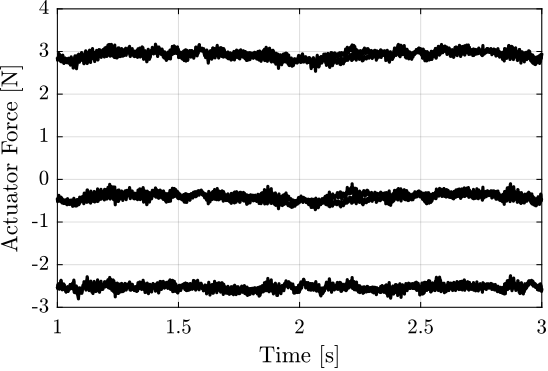
Figure 65: Forces applied by the six nano-hexapod’s actuators
The relative motions of the nano-hexapod’s legs is shown in Figure 66 and are in the micro-meter range.
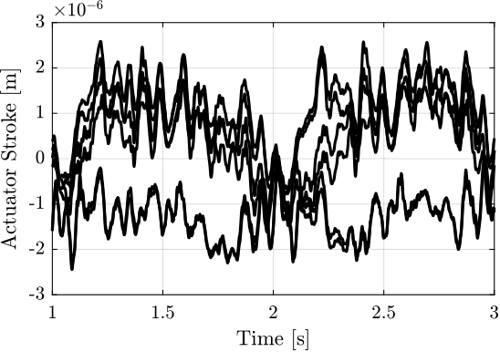
Figure 66: Relative displacement of the nano-hexapod’s legs
Finally, the position/orientation error of the sample is shown in Figure 67. The root mean square value of the x-y-z error motions is around \(30\,nm\) which is very similar than for the “simple” tomography experiment.
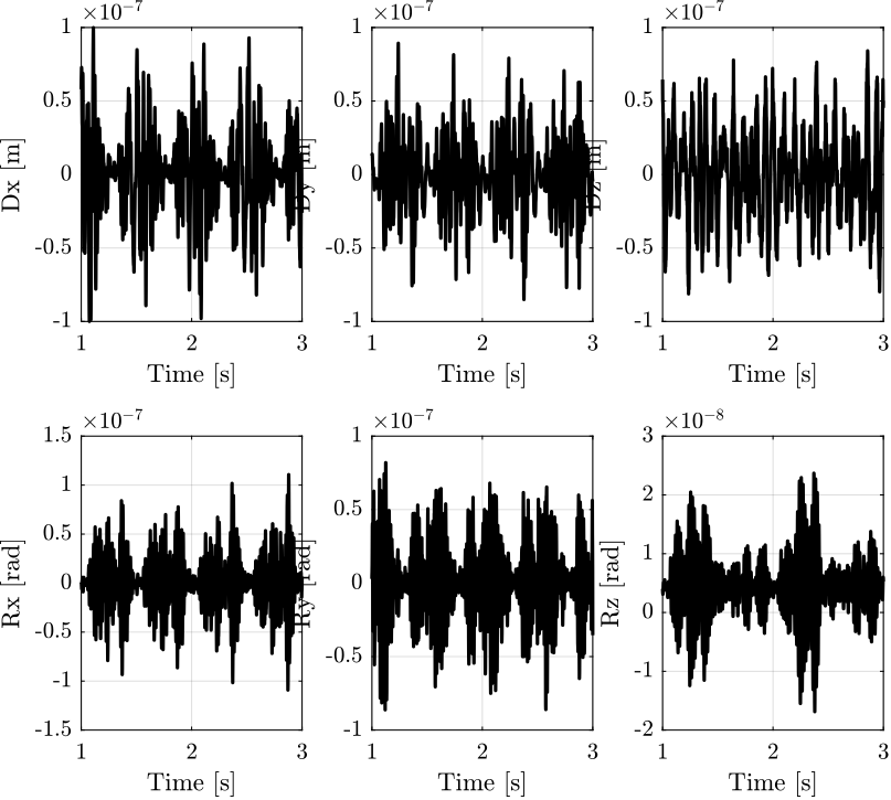
Figure 67: Position/orientation error of the sample during the simulation
Simultaneous Translation Scans and Spindle’s rotation
In this simulation:
- the sample has a mass of 1kg
- the spindle rotation speed is set to 60rpm
- scans with the translation stage are performed simultaneously with a triangular shape having a period of 4s and an amplitude of 5mm
The obtained sample’s motion during the simulation is shown in Figure 68.

Figure 68: Top View of a tomography experiment combined with translation scans
The forces applied by the nano-hexapod’s are shown in Figure 69. Peak values of the forces are appearing when the translation stage changes the direction of the scan.
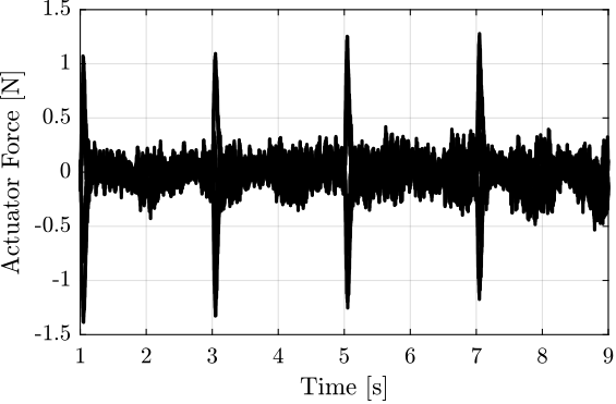
Figure 69: Forces applied by the six nano-hexapod’s actuators
The relative motions of the nano-hexapod’s legs is shown in Figure 70 and are again in the micro-meter range.
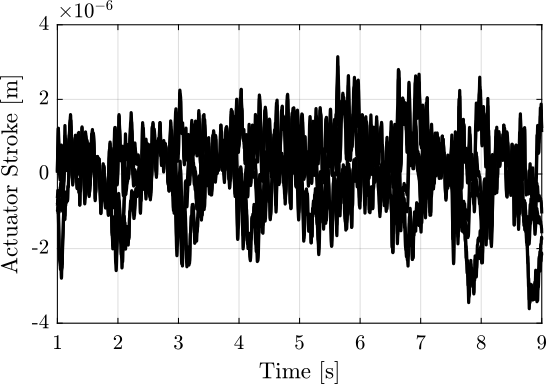
Figure 70: Relative displacement of the nano-hexapod’s legs
The time domain position/orientation error of the sample is shown in Figure 71. The RMS value of the x-y-z position error is again \(\approx 30\,nm\).
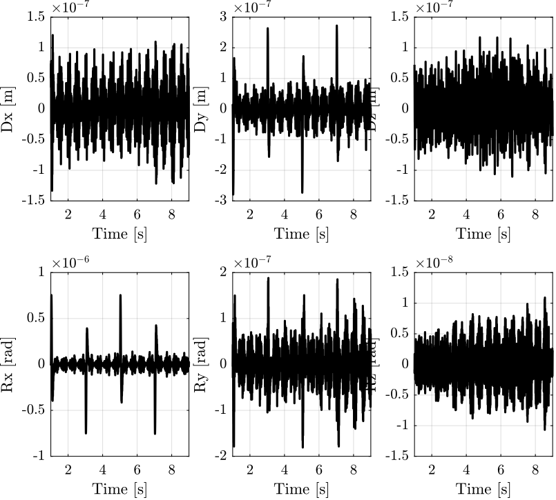
Figure 71: Position/orientation error of the sample during the simulation
Conclusion
These two simulations of more complex experiments shows the robustness of the developed system.
Indeed, the obtained performances are very similar for all three simulated experiments.
The required actuator stroke is shown to be around \(\pm 5\,\mu m\) to compensate the dynamical errors, and the required actuators forces remain small.
6.6 Conclusion
The High Authority Control / Low Authority Control architecture has been implemented in the multi-body model of the NASS.
It consists of a Direct Velocity Feedback control used to damp the nano-hexapod resonances and an outer controller designed in the space of the legs to lower the effect of disturbances.
Relative motion sensors should be included in each of the nano-hexapod’s leg for active damping purposes. The best sensor technology should further be determined based on cost, ease of integration, bandwidth and resolution. Possible technologies include capacitive sensors, eddy current sensors and encoders.
The control architecture used is shown to lower the effect of disturbances up to 100Hz and appears to be very robust to all considered changes in the system.
Simulations performed in presence of ground motion and stage vibrations gives an obtained residual X-Y-Z sample’s vibrations around \(30\,[nm]\,rms\).
The simulation is considered to be fairly realistic as the model used has been show to properly represents the micro-station dynamics and the disturbances included were based on measurements.
Further optimization of the control architecture are foreseen to give better performance.
7 General Conclusion and Further notes
A summary of the nano-hexapod specifications is given in Section 7.1.
In section 7.2 is explained why the metrology was supposed to be perfect during the simulation and how to account from measurement imperfections. In section 7.3, disturbance sources that were not included in the model are discussed.
The problem of static deflection when changing the payload is discussed in Section 7.4.
If ground motion is found to be the limiting factor, soft mounts can be used for the granite. This is discussed in Section 7.6.
Finally, some notes about the Micro-Station are drawn in Section 7.5.
7.1 Nano-Hexapod Specifications
Dimensions
The wanted dimension of the nano-hexapod are shown in Figure 72:
- Diameter of the bottom platform: 300mm
- Diameter of the top platform: 200mm
- Maximum Height: 90mm
The limiting height might be quite problematic for the integration of the flexible joints, the actuators and sensors.
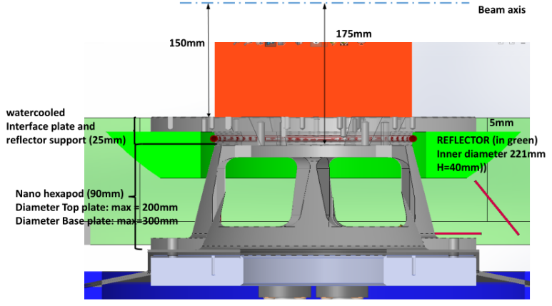
Figure 72: First implementation of the nano-hexapod / metrology reflector and sample interface
Flexible Joints
Flexible joints are located at each end of the six struts. These flexible joints should have the following properties:
- High Axial Stiffness: \(K_a > 10^7\,[N/m]\)
- Small Bending Stiffness: \(K_b < 50\,[Nm/rad]\)
- Small Torsion Stiffness: \(K_t < 50\,[Nm/rad]\)
The required angular stroke has not been estimated in this study. It is however simple to do so as the angular motion of each joint can easily be measured in the multi-body model used to perform the simulations. Typical angular stroke for such flexible joints is expected.
Strut Stiffness
The axial stiffness of the struts (between two flexible joints) should be equal to \(\approx 10^5 - 10^6\,[N/m]\).
If voice coils are used, this corresponds to the axial stiffness of the membrane guiding the moving part of the voice coil.
Actuator Force
Based on simulations:
- Continuous Force: \(\pm 5\,[N]\) (due to centrifugal forces)
- “Variable” Force: \(\pm 1\,[N]\)
If static deflection is to be compensated by the actuator, \(\approx 100\,[N]\) of continuous force is required for each actuator.
Actuator Stroke
Based on simulations, the required actuator stroke seems to be \(\pm 5\,[\mu m]\).
This however does not take into account two error types that will have to be compensated by the nano-hexapod:
- the static positioning errors of all the micro-station’s stages. These errors have been measured by Hans-Peter, and are in the order of tens of \(\mu m\) and tens of \(\mu rad\).
- the tracking errors of the translation stage and tilt stage. This is probably more difficult to estimate. However, by limiting the acceleration of these stages, we may limit the dynamic tracking errors to acceptable levels
Some security margin should be taken as if the nano-hexapod has not enough stroke to compensated the above errors, the system will not be able to compensate all the vibrations.
Thus, an actuator stroke of \(\pm 50 \mu m\) would be quite safe.
Note that a piezoelectric stack have a maximum strain of \(0.1\%\). A piezo stack with a stroke of \(\pm 50\,[\mu m]\) will have a length size of \(\approx 100\,[mm]\) making it difficult to integrate in the nano-hexapod.
Some amplified piezoelectric actuators that fulfill the requirements are listed in Table 5. The actuators that seems the most suited will be modeled using a FE software and integrated into the Simscape model as explained in Section 5.5. Simulation will be performed with the chosen actuator to make sure that the obtained performance is acceptable.
| Specification | APA150M | APA400MML | APA300ML | FPA-0500E-P-1036 | FPA-0300E-S-0536 | FPA-0150E-S-0518 | |
|---|---|---|---|---|---|---|---|
| Stroke | \(> 100\, [\mu m]\) | 187 | 368 | 304 | 432 | 240 | 132 |
| Stiffness | \(0.1-1\, [N/\mu m]\) | 0.7 | 0.55 | 1.8 | 0.87 | 0.58 | 0.8 |
| Resolution | \(< 2\, [nm]\) | 2 | 4 | 3 | |||
| Blocked Force | \(> 100\, [N]\) | 127 | 201 | 546 | 376 | 139 | 106 |
| Height | \(< 50\, [mm]\) | 22 | 24 | 30 | 27 | 16 | 15 |
| Price | 2300$ | 1400$ | 890$ |
Sensors
A relative displacement sensor must be included in each of the nano-hexapod’s legs as explained in Section 6.
The sensors must as the following properties:
- High bandwidth \(> 1\,[kHz]\)
- Fine resolution \(< 10\,[nm]\)
- Range of \(> 100\,[\mu m]\)
Note that the sensor signal will have to pass through the Slip-Ring. This adds few constrains:
- The sensor signal must be immune to some “electrical noise” that could be induced by the slip-ring
- Limited number of slip-ring channels should be required for the six sensors
Several sensor technology could be used for the nano-hexapod. Characteristics of those sensors are shown in Table 6.
| Technology | Frequency | Resolution | Range | T Range |
|---|---|---|---|---|
| LVDT | DC-200 Hz | 10 nm rms | 1-10 mm | -50,100 °C |
| Eddy current | 5 kHz | 0.1-100 nm rms | 0.5-55 mm | -50,100 °C |
| Capacitive | DC-100 kHz | 0.05-50 nm rms | 50 nm - 1 cm | -40,100 °C |
| Interferometer | 300 kHz | 0.1 nm rms | 10 cm | -250,100 °C |
| Encoder | DC-1 MHz | 1 nm rms | 7-27 mm | 0,40 °C |
Two sensor technologies seem the most adapted to the nano-hexapod: the eddy current sensor and the capacitive sensor. They both exhibit few nanometers of resolution over a stroke of \(100\,[\mu m]\) and a sufficient bandwidth.
Cedrat proposes to integrate Eddy Current Sensors in their amplified piezoelectric actuator as shown in Figure 73. An alternative could be to use the capacitive sensors such as the very compact D-100 proposed by PI.
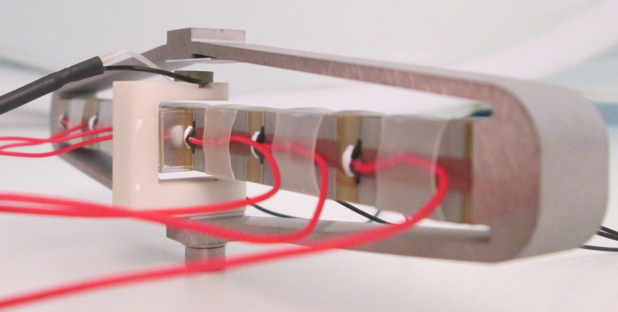
Figure 73: Eddy Current Sensors integrated into a Cedrat’s amplified piezoelectric actuator
Architecture
As explained in section 5.4 the orientation of the legs and position of the joints are very much constrained by the limited height of the nano-hexapod.
7.2 Sensor Noise introduced by the Metrology
During all this study, the measurement of the relative position of the sample with respect to the granite was considered to be perfect, that is to say noiseless and with infinite bandwidth.
This was done for the following reasons:
- interferometers have such a large bandwidth (> MHz) compared to the control bandwidth (\(\approx 100\,[Hz]\)) that their dynamics can indeed be considered to be represented by “unit transfer functions”
- sensor noise can generally be considered separately. As a matter of fact, the sensor noise is completely transmitted to the sample’s motion within the control bandwidth and is filtered outside the control bandwidth. It is then quite simple to predict what will be the effect of the sensor noise on the sample’s motion.
7.3 Others Factors that may limit the performances
Many sources of noise and perturbation were not taken into account in this study:
- Cable forces applied on the Sample
- Electronic noise induced by the Slip-Ring
- Measurement noise of the metrology system (discussed in Section 7.2)
- Electronic noise of the amplifiers used for the actuators
- Noise of the relative motion sensor included in the nano-hexapod
- ADC and DAC quantization noise and electronic noise
- Acoustic Noise, Brownian noise, turbulence, …
Thanks to the noise budgeting, it is quite easy to determine the required characteristics of the ADC, DAC, sensors and amplifiers such that they do not limit the performances of the system.
Further tests should be done in order to ensure that the slip-ring will not add significant noise to both the sensors and actuators included in the nano-hexapod.
If heavy/stiff cables are fixed to the sample, this can:
- induced vibrations way above specification
- change the dynamics of the nano-hexapod and limit the attainable bandwidth
As cable forces are often the limiting factor in high precision mechatronic systems, this have to be carefully taken into account during the mechanical design of the nano-hexapod.
7.4 Static Deflection
Let’s now consider the problem of static deflection when changing the payload.
The maximum payload’s mass is \(50\,[kg]\), this corresponds to an added vertical force of \(\approx 500\,[N]\).
If this is to be compensated by the nano-hexapod, \(\approx 100\,[N]\) should be applied by each of the nano-hexapod’s actuators. In such case, the nano-hexapod keeps its nominal configuration.
In practice, this could be done using the relative motion sensor included in each leg, and a feedback control keeping the legs displacements at the wanted value.
This might not be a problem is piezoelectric stacks are used, but it is a big issue is voice coils are used.
An alternative would be to accept that the nano-hexapod experiences some static deflection.
With a vertical nano-hexapod stiffness \(\approx 10^6\,[N/m]\), the maximum static deflection would be: \[ k_z \approx 10^6\,[N/m] \longrightarrow \Delta z = \frac{\Delta m g}{k_z} \approx 0.5\,[mm] \] This will change a little bit the architecture of the nano-hexapod but this should be too small to change significantly the dynamics.
7.5 Micro Station Architecture
The micro-station impacts the performance of the NASS mainly because of vibrations induced by its imperfect mechanics.
The micro-station has also an impact on the design of nano-hexapod:
- its absolute position accuracy determine the required nano-hexapod mobility (stroke)
- its dynamics (mainly frequency of the first mode) impose an upper limit for the stiffness of the nano-hexapod
Other than that, the NASS is mostly independent of the micro-station and could be used on top of other positioning end stations.
Some notes about an alternative micro-station architecture are accessible here.
7.6 Using soft mounts for the Granite
If it is found that ground motion is what is limiting the system performances, an option is to support the granite on soft mounts.
These soft mounts can topically consists of air cylinders with pistons guided by air bearings.
The suspension mode of the granite would then be in the order of few Hertz, and the ground motion would be filtered out above that frequency as shown in Figure 74.
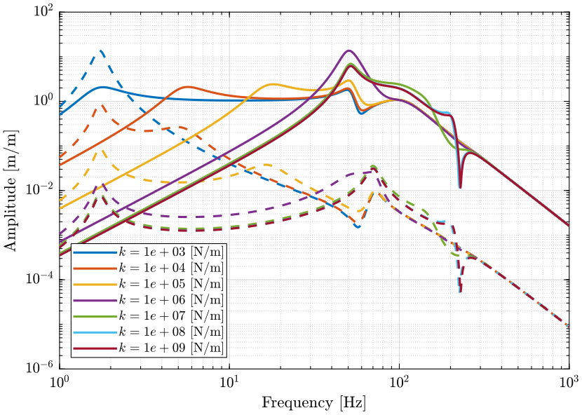
Figure 74: Change of sensibility to Ground motion when using stiff Granite mounts (solid curves) and soft Granite mounts (dashed curves)
7.7 General Conclusion
The main outcome of this study is a series of specifications for the nano-hexapod. These specifications seems realistic, and a detailed mechanical design of the nano-hexapod can be initiated.
A robust control architecture has been developed and implemented in the model. Further work on the control side should be performed using more advanced robust techniques. This is foreseen to give better performances and robustness.
Realistic simulations of scientific experiments were carried out validating the concept.