Active Damping of Rotating Platforms using Integral Force Feedback - Matlab Computation

Table of ContentsClose

1. System Description and Analysis
2. Problem with pure Integral Force Feedback
3. Integral Force Feedback with an High Pass Filter
4. IFF with a stiffness in parallel with the force sensor
5. Comparison
6. Notations

This report is also available as a pdf.

This document gathers the Matlab code used to for the conference paper (Dehaeze and Collette 2020) and the journal paper (Dehaeze and Collette 2021).

It is structured in several sections:

Section 1: presents a simple model of a rotating suspended platform that will be used throughout this study.
Section 2: explains how the unconditional stability of IFF is lost due to Gyroscopic effects induced by the rotation.
Section 3: suggests a simple modification of the control law such that damping can be added to the suspension modes in a robust way.
Section 4: proposes to add springs in parallel with the force sensors to regain the unconditional stability of IFF.
Section 5: compares both proposed modifications to the classical IFF in terms of damping authority and closed-loop system behavior.
Section 6: contains the notations used for both the Matlab code and the paper

The matlab code is accessible on Zonodo and Github (Dehaeze 2020). It can also be download as a .zip file here.

To run the Matlab code, go in the matlab directory and run the following Matlab files corresponding to each section.

Table 1: Paper’s sections and corresponding Matlab files
Sections	Matlab File
Section 1	`s1_system_description.m`
Section 2	`s2_iff_pure_int.m`
Section 3	`s3_iff_hpf.m`
Section 4	`s4_iff_kp.m`
Section 5	`s5_act_damp_comparison.m`

1 System Description and Analysis

1.1 System description

The system consists of one 2 degree of freedom translation stage on top of a spindle (figure 1).

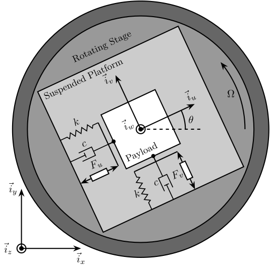
Figure 1: Schematic of the studied system

The control inputs are the forces applied by the actuators of the translation stage ( $F_{u}$ and $F_{v}$ ). As the translation stage is rotating around the Z axis due to the spindle, the forces are applied along ${\vec{i}}_{u}$ and ${\vec{i}}_{v}$ .

1.2 Equations

Based on the Figure 1, the equations of motions are:

Important

\begin{matrix} (1) & [\begin{matrix} d_{u} \\ d_{v} \end{matrix}] = G_{d} [\begin{matrix} F_{u} \\ F_{v} \end{matrix}] \end{matrix}

Where $G_{d}$ is a $2 \times 2$ transfer function matrix.

\begin{matrix} (2) & G_{d} = \frac{1}{k} \frac{1}{G_{d p}} [\begin{matrix} G_{d z} & G_{d c} \\ - G_{d c} & G_{d z} \end{matrix}] \end{matrix}

With:

\begin{aligned} (3) & G_{d p} & = {(\frac{s^{2}}{{ω_{0}}^{2}} + 2 ξ \frac{s}{ω_{0}} + 1 - \frac{Ω^{2}}{{ω_{0}}^{2}})}^{2} + {(2 \frac{Ω}{ω_{0}} \frac{s}{ω_{0}})}^{2} \\ (4) & G_{d z} & = \frac{s^{2}}{{ω_{0}}^{2}} + 2 ξ \frac{s}{ω_{0}} + 1 - \frac{Ω^{2}}{{ω_{0}}^{2}} \\ (5) & G_{d c} & = 2 \frac{Ω}{ω_{0}} \frac{s}{ω_{0}} \end{aligned}

1.3 Numerical Values

Let’s define initial values for the model.

Copy
  k = 1;    % Actuator Stiffness [N/m]
  c = 0.05; % Actuator Damping [N/(m/s)]
  m = 1;    % Payload mass [kg]

Copy
  xi = c/(2*sqrt(k*m));
  w0 = sqrt(k/m); % [rad/s]

1.4 Campbell Diagram

The Campbell Diagram displays the evolution of the real and imaginary parts of the system as a function of the rotating speed.

It is shown in Figures 2 and 3, and one can see that the system becomes unstable for $Ω > ω_{0}$ (the real part of one of the poles becomes positive).

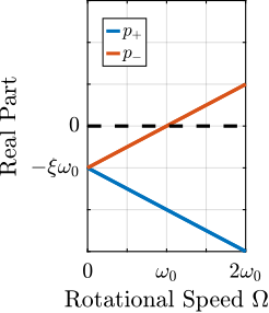
Figure 2: Campbell Diagram - Real Part

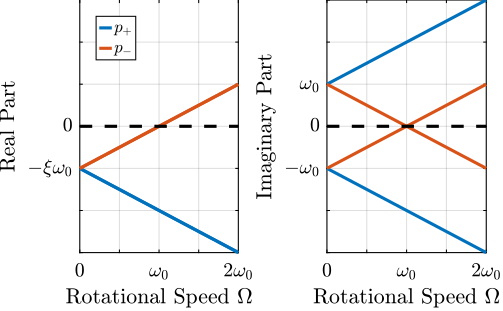
Figure 3: Campbell Diagram - Imaginary Part

1.5 Simscape Model

In order to validate all the equations of motion, a Simscape model of the same system has been developed. The dynamics of the system can be identified from the Simscape model and compare with the analytical model.

The rotating speed for the Simscape Model is defined.

Copy
  W = 0.1; % Rotation Speed [rad/s]

Copy
  open('rotating_frame.slx');

The transfer function from $[F_{u}, F_{v}]$ to $[d_{u}, d_{v}]$ is identified from the Simscape model.

Copy
  %% Name of the Simulink File
  mdl = 'rotating_frame';

  %% Input/Output definition
  clear io; io_i = 1;
  io(io_i) = linio([mdl, '/K'], 1, 'openinput');  io_i = io_i + 1;
  io(io_i) = linio([mdl, '/G'], 2, 'openoutput'); io_i = io_i + 1;

Copy  G = linearize(mdl, io, 0);

  %% Input/Output definition
  G.InputName  = {'Fu', 'Fv'};
  G.OutputName = {'du', 'dv'};

The same transfer function from $[F_{u}, F_{v}]$ to $[d_{u}, d_{v}]$ is written down from the analytical model.

Copy
  Gth = (1/k)/(((s^2)/(w0^2) + 2*xi*s/w0 + 1 - (W^2)/(w0^2))^2 + (2*W*s/(w0^2))^2) * ...
        [(s^2)/(w0^2) + 2*xi*s/w0 + 1 - (W^2)/(w0^2), 2*W*s/(w0^2) ; ...
         -2*W*s/(w0^2), (s^2)/(w0^2) + 2*xi*s/w0 + 1 - (W^2)/(w0^2)];

Both transfer functions are compared in Figure 4 and are found to perfectly match.

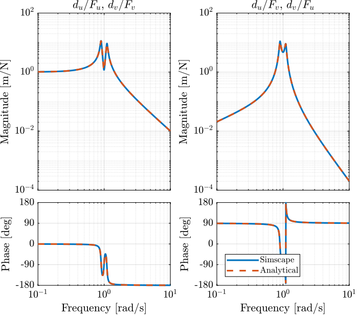
Figure 4: Bode plot of the transfer function from $[F_{u}, F_{v}]$ to $[d_{u}, d_{v}]$ as identified from the Simscape model and from an analytical model

1.6 Effect of the rotation speed

The transfer functions from $[F_{u}, F_{v}]$ to $[d_{u}, d_{v}]$ are identified for the following rotating speeds.

Copy
  Ws = [0, 0.2, 0.7, 1.1]*w0; % Rotating Speeds [rad/s]

Copy  Gs = {zeros(2, 2, length(Ws))};

  for W_i = 1:length(Ws)
      W = Ws(W_i);

      Gs(:, :, W_i) = {(1/k)/(((s^2)/(w0^2) + 2*xi*s/w0 + 1 - (W^2)/(w0^2))^2 + (2*W*s/(w0^2))^2) * ...
                       [(s^2)/(w0^2) + 2*xi*s/w0 + 1 - (W^2)/(w0^2), 2*W*s/(w0^2) ; ...
                        -2*W*s/(w0^2), (s^2)/(w0^2) + 2*xi*s/w0 + 1 - (W^2)/(w0^2)]};
  end

They are compared in Figures 5 and 6.

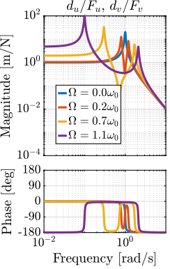
Figure 5: Comparison of the transfer functions from $[F_{u}, F_{v}]$ to $[d_{u}, d_{v}]$ for several rotating speed - Direct Terms

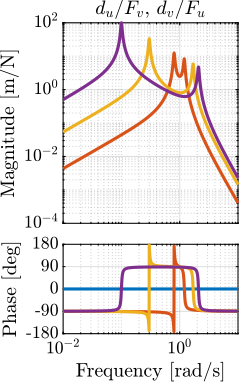
Figure 6: Comparison of the transfer functions from $[F_{u}, F_{v}]$ to $[d_{u}, d_{v}]$ for several rotating speed - Coupling Terms

2 Problem with pure Integral Force Feedback

Force sensors are added in series with the two actuators (Figure 7).

Two identical controllers $K_{F}$ are used to feedback each of the sensed force to its associated actuator.

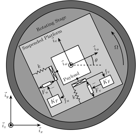
Figure 7: System with added Force Sensor in series with the actuators

2.1 Plant Parameters

Let’s define initial values for the model.

Copy
  k = 1;    % Actuator Stiffness [N/m]
  c = 0.05; % Actuator Damping [N/(m/s)]
  m = 1;    % Payload mass [kg]

Copy
  xi = c/(2*sqrt(k*m));
  w0 = sqrt(k/m); % [rad/s]

2.2 Equations

The sensed forces are equal to:

\begin{matrix} (6) & [\begin{matrix} f_{u} \\ f_{v} \end{matrix}] = [\begin{matrix} 1 & 0 \\ 0 & 1 \end{matrix}] [\begin{matrix} F_{u} \\ F_{v} \end{matrix}] - (c s + k) [\begin{matrix} d_{u} \\ d_{v} \end{matrix}] \end{matrix}

Which then gives:

Important

\begin{matrix} (7) & [\begin{matrix} f_{u} \\ f_{v} \end{matrix}] = G_{f} [\begin{matrix} F_{u} \\ F_{v} \end{matrix}] \end{matrix}

\begin{matrix} (8) & [\begin{matrix} f_{u} \\ f_{v} \end{matrix}] = \frac{1}{G_{f p}} [\begin{matrix} G_{f z} & - G_{f c} \\ G_{f c} & G_{f z} \end{matrix}] [\begin{matrix} F_{u} \\ F_{v} \end{matrix}] \end{matrix}

\begin{aligned} (9) & G_{f p} & = {(\frac{s^{2}}{{ω_{0}}^{2}} + 2 ξ \frac{s}{ω_{0}} + 1 - \frac{Ω^{2}}{{ω_{0}}^{2}})}^{2} + {(2 \frac{Ω}{ω_{0}} \frac{s}{ω_{0}})}^{2} \\ (10) & G_{f z} & = (\frac{s^{2}}{{ω_{0}}^{2}} - \frac{Ω^{2}}{{ω_{0}}^{2}}) (\frac{s^{2}}{{ω_{0}}^{2}} + 2 ξ \frac{s}{ω_{0}} + 1 - \frac{Ω^{2}}{{ω_{0}}^{2}}) + {(2 \frac{Ω}{ω_{0}} \frac{s}{ω_{0}})}^{2} \\ (11) & G_{f c} & = (2 ξ \frac{s}{ω_{0}} + 1) (2 \frac{Ω}{ω_{0}} \frac{s}{ω_{0}}) \end{aligned}

2.3 Comparison of the Analytical Model and the Simscape Model

The rotation speed is set to $Ω = 0.1 ω_{0}$ .

Copy
  W = 0.1*w0; % [rad/s]

Copy
  open('rotating_frame.slx');

And the transfer function from $[F_{u}, F_{v}]$ to $[f_{u}, f_{v}]$ is identified using the Simscape model.

Copy
  %% Name of the Simulink File
  mdl = 'rotating_frame';

  %% Input/Output definition
  clear io; io_i = 1;
  io(io_i) = linio([mdl, '/K'], 1, 'openinput');  io_i = io_i + 1;
  io(io_i) = linio([mdl, '/G'], 1, 'openoutput'); io_i = io_i + 1;

Copy  Giff = linearize(mdl, io, 0);

  %% Input/Output definition
  Giff.InputName  = {'Fu', 'Fv'};
  Giff.OutputName = {'fu', 'fv'};

The same transfer function from $[F_{u}, F_{v}]$ to $[f_{u}, f_{v}]$ is written down from the analytical model.

Copy
  Giff_th = 1/(((s^2)/(w0^2) + 2*xi*s/w0 + 1 - (W^2)/(w0^2))^2 + (2*W*s/(w0^2))^2) * ...
            [(s^2/w0^2 - W^2/w0^2)*((s^2)/(w0^2) + 2*xi*s/w0 + 1 - (W^2)/(w0^2)) + (2*W*s/(w0^2))^2, - (2*xi*s/w0 + 1)*2*W*s/(w0^2) ; ...
             (2*xi*s/w0 + 1)*2*W*s/(w0^2), (s^2/w0^2 - W^2/w0^2)*((s^2)/(w0^2) + 2*xi*s/w0 + 1 - (W^2)/(w0^2))+ (2*W*s/(w0^2))^2];

The two are compared in Figure 8 and found to perfectly match.

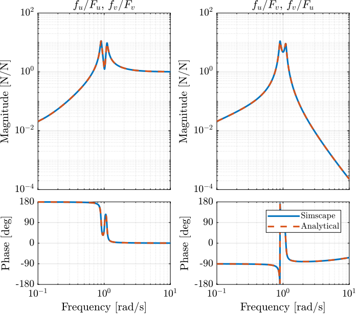
Figure 8: Comparison of the transfer functions from $[F_{u}, F_{v}]$ to $[f_{u}, f_{v}]$ between the Simscape model and the analytical one

2.4 Effect of the rotation speed

The transfer functions from $[F_{u}, F_{v}]$ to $[f_{u}, f_{v}]$ are identified for the following rotating speeds.

Copy
  Ws = [0, 0.2, 0.7]*w0; % Rotating Speeds [rad/s]

Copy  Gsiff = {zeros(2, 2, length(Ws))};

  for W_i = 1:length(Ws)
      W = Ws(W_i);

      Gsiff(:, :, W_i) = {1/(((s^2)/(w0^2) + 2*xi*s/w0 + 1 - (W^2)/(w0^2))^2 + (2*W*s/(w0^2))^2) * ...
                        [(s^2/w0^2 - W^2/w0^2)*((s^2)/(w0^2) + 2*xi*s/w0 + 1 - (W^2)/(w0^2)) + (2*W*s/(w0^2))^2, - (2*xi*s/w0 + 1)*2*W*s/(w0^2) ; ...
                         (2*xi*s/w0 + 1)*2*W*s/(w0^2), (s^2/w0^2 - W^2/w0^2)*((s^2)/(w0^2) + 2*xi*s/w0 + 1 - (W^2)/(w0^2))+ (2*W*s/(w0^2))^2]};
  end

The obtained transfer functions are shown in Figure 9.

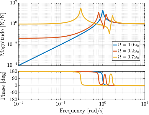
Figure 9: Comparison of the transfer functions from $[F_{u}, F_{v}]$ to $[f_{u}, f_{v}]$ for several rotating speed

2.5 Decentralized Integral Force Feedback

The decentralized IFF controller consists of pure integrators:

\begin{matrix} (12) & K_{IFF} (s) = \frac{g}{s} [\begin{matrix} 1 & 0 \\ 0 & 1 \end{matrix}] \end{matrix}

The Root Locus (evolution of the poles of the closed loop system in the complex plane as a function of $g$ ) is shown in Figure 10. It is shown that for non-null rotating speed, one pole is bound to the right-half plane, and thus the closed loop system is unstable.

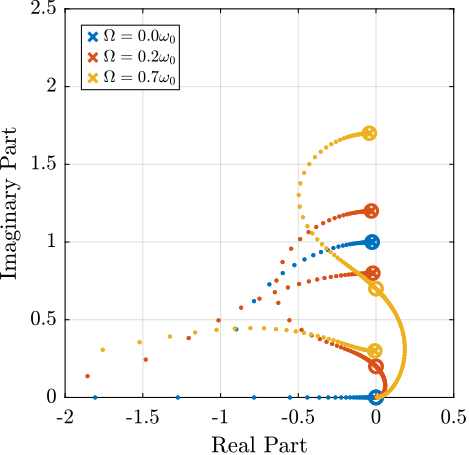
Figure 10: Root Locus for the Decentralized Integral Force Feedback controller. Several rotating speed are shown.

3 Integral Force Feedback with an High Pass Filter

3.1 Plant Parameters

Let’s define initial values for the model.

Copy
  k = 1;    % Actuator Stiffness [N/m]
  c = 0.05; % Actuator Damping [N/(m/s)]
  m = 1;    % Payload mass [kg]

Copy
  xi = c/(2*sqrt(k*m));
  w0 = sqrt(k/m); % [rad/s]

3.2 Modified Integral Force Feedback Controller

Let’s modify the initial Integral Force Feedback Controller ; instead of using pure integrators, pseudo integrators (i.e. low pass filters) are used:

\begin{matrix} (13) & K_{IFF} (s) = g \frac{1}{ω_{i} + s} [\begin{matrix} 1 & 0 \\ 0 & 1 \end{matrix}] \end{matrix}

where $ω_{i}$ characterize down to which frequency the signal is integrated.

Let’s arbitrary choose the following control parameters:

Copy  g = 2;
  wi = 0.1*w0;

And the following rotating speed.

Copy
  Giff = 1/(((s^2)/(w0^2) + 2*xi*s/w0 + 1 - (W^2)/(w0^2))^2 + (2*W*s/(w0^2))^2) * ...
          [(s^2/w0^2 - W^2/w0^2)*((s^2)/(w0^2) + 2*xi*s/w0 + 1 - (W^2)/(w0^2)) + (2*W*s/(w0^2))^2, - (2*xi*s/w0 + 1)*2*W*s/(w0^2) ; ...
           (2*xi*s/w0 + 1)*2*W*s/(w0^2), (s^2/w0^2 - W^2/w0^2)*((s^2)/(w0^2) + 2*xi*s/w0 + 1 - (W^2)/(w0^2))+ (2*W*s/(w0^2))^2];

The obtained Loop Gain is shown in Figure 11.

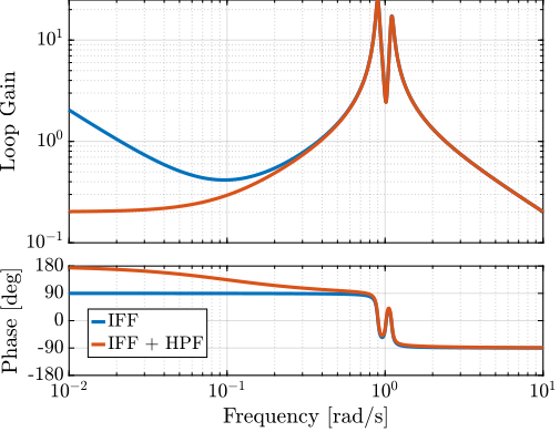
Figure 11: Loop Gain for the modified IFF controller

3.3 Root Locus

As shown in the Root Locus plot (Figure 12), for some value of the gain, the system remains stable.

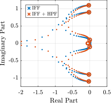
Figure 12: Root Locus for the modified IFF controller

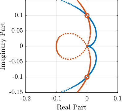
Figure 13: Root Locus for the modified IFF controller - Zoom

3.4 What is the optimal $ω_{i}$ and $g$ ?

In order to visualize the effect of $ω_{i}$ on the attainable damping, the Root Locus is displayed in Figure 14 for the following $ω_{i}$ :

Copy
  wis = [0.01, 0.1, 0.5, 1]*w0; % [rad/s]

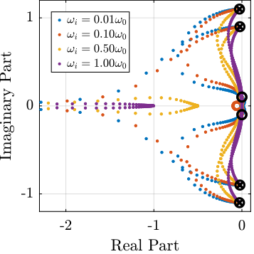
Figure 14: Root Locus for the modified IFF controller (zoomed plot on the left)

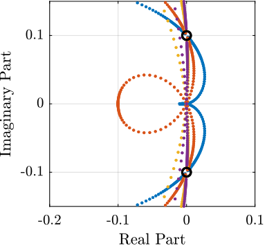
Figure 15: Root Locus for the modified IFF controller (zoomed plot on the left)

For the controller

\begin{matrix} (14) & K_{IFF} (s) = g \frac{1}{ω_{i} + s} [\begin{matrix} 1 & 0 \\ 0 & 1 \end{matrix}] \end{matrix}

The gain at which the system becomes unstable is

\begin{matrix} (15) & g_{max} = ω_{i} (\frac{{ω_{0}}^{2}}{Ω^{2}} - 1) \end{matrix}

While it seems that small $ω_{i}$ do allow more damping to be added to the system (Figure 14), the control gains may be limited to small values due to $(15)$ thus reducing the attainable damping.

There must be an optimum for $ω_{i}$ . To find the optimum, the gain that maximize the simultaneous damping of the mode is identified for a wide range of $ω_{i}$ (Figure 16).

Copy
  wis = logspace(-2, 1, 100)*w0; % [rad/s]

  opt_xi = zeros(1, length(wis)); % Optimal simultaneous damping
  opt_gain = zeros(1, length(wis)); % Corresponding optimal gain

  for wi_i = 1:length(wis)
      wi = wis(wi_i);
      Kiff = 1/(s + wi)*eye(2);

      fun = @(g)computeSimultaneousDamping(g, Giff, Kiff);

      [g_opt, xi_opt] = fminsearch(fun, 0.5*wi*((w0/W)^2 - 1));
      opt_xi(wi_i) = 1/xi_opt;
      opt_gain(wi_i) = g_opt;
  end

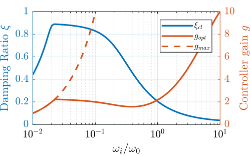
Figure 16: Simultaneous attainable damping of the closed loop poles as a function of $ω_{i}$

4 IFF with a stiffness in parallel with the force sensor

4.1 Schematic

In this section additional springs in parallel with the force sensors are added to counteract the negative stiffness induced by the rotation.

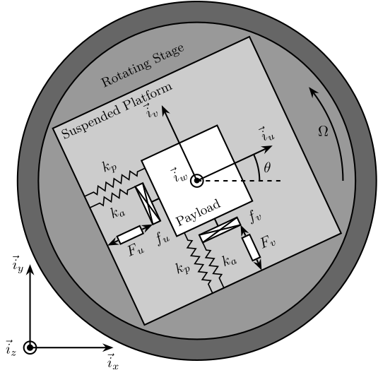
Figure 17: Studied system with additional springs in parallel with the actuators and force sensors

In order to keep the overall stiffness $k = k_{a} + k_{p}$ constant, a scalar parameter $α$ ( $0 \leq α < 1$ ) is defined to describe the fraction of the total stiffness in parallel with the actuator and force sensor

\begin{matrix} (16) & k_{p} = α k, k_{a} = (1 - α) k \end{matrix}

4.2 Equations

Important

\begin{matrix} (17) & [\begin{matrix} f_{u} \\ f_{v} \end{matrix}] = G_{k} [\begin{matrix} F_{u} \\ F_{v} \end{matrix}] \end{matrix}

\begin{matrix} (18) & [\begin{matrix} f_{u} \\ f_{v} \end{matrix}] = \frac{1}{G_{k p}} [\begin{matrix} G_{k z} & - G_{k c} \\ G_{k c} & G_{k z} \end{matrix}] [\begin{matrix} F_{u} \\ F_{v} \end{matrix}] \end{matrix}

With:

\begin{aligned} (19) & G_{k p} & = {(\frac{s^{2}}{{ω_{0}}^{2}} + 2 ξ \frac{s}{{ω_{0}}^{2}} + 1 - \frac{Ω^{2}}{{ω_{0}}^{2}})}^{2} + {(2 \frac{Ω}{ω_{0}} \frac{s}{ω_{0}})}^{2} \\ (20) & G_{k z} & = (\frac{s^{2}}{{ω_{0}}^{2}} - \frac{Ω^{2}}{{ω_{0}}^{2}} + α) (\frac{s^{2}}{{ω_{0}}^{2}} + 2 ξ \frac{s}{{ω_{0}}^{2}} + 1 - \frac{Ω^{2}}{{ω_{0}}^{2}}) + {(2 \frac{Ω}{ω_{0}} \frac{s}{ω_{0}})}^{2} \\ (21) & G_{k c} & = (2 ξ \frac{s}{ω_{0}} + 1 - α) (2 \frac{Ω}{ω_{0}} \frac{s}{ω_{0}}) \end{aligned}

If we compare $G_{k z}$ and $G_{f z}$ , we see that the spring in parallel adds a term $α$ . In order to have two complex conjugate zeros (instead of real zeros):

\begin{matrix} (22) & α > \frac{Ω^{2}}{{ω_{0}}^{2}} \Leftrightarrow k_{p} > m Ω^{2} \end{matrix}

4.3 Plant Parameters

Let’s define initial values for the model.

Copy
  k = 1;    % Actuator Stiffness [N/m]
  c = 0.05; % Actuator Damping [N/(m/s)]
  m = 1;    % Payload mass [kg]

Copy
  xi = c/(2*sqrt(k*m));
  w0 = sqrt(k/m); % [rad/s]

4.4 Comparison of the Analytical Model and the Simscape Model

The same transfer function from $[F_{u}, F_{v}]$ to $[f_{u}, f_{v}]$ is written down from the analytical model.

Copy
  W = 0.1*w0; % [rad/s]

  kp = 1.5*m*W^2;
  cp = 0;

Copy
  open('rotating_frame.slx');

Copy
  %% Name of the Simulink File
  mdl = 'rotating_frame';

  %% Input/Output definition
  clear io; io_i = 1;
  io(io_i) = linio([mdl, '/K'], 1, 'openinput');  io_i = io_i + 1;
  io(io_i) = linio([mdl, '/G'], 1, 'openoutput'); io_i = io_i + 1;

  Giff = linearize(mdl, io, 0);

  %% Input/Output definition
  Giff.InputName  = {'Fu', 'Fv'};
  Giff.OutputName = {'fu', 'fv'};

Copy
  w0p = sqrt((k + kp)/m);
  xip = c/(2*sqrt((k+kp)*m));

  Giff_th = 1/( (s^2/w0p^2 + 2*xip*s/w0p + 1 - W^2/w0p^2)^2 + (2*(s/w0p)*(W/w0p))^2 ) * [ ...
                     (s^2/w0p^2 + kp/(k + kp) - W^2/w0p^2)*(s^2/w0p^2 + 2*xip*s/w0p + 1 - W^2/w0p^2) + (2*(s/w0p)*(W/w0p))^2, -(2*xip*s/w0p + k/(k + kp))*(2*(s/w0p)*(W/w0p));
                     (2*xip*s/w0p + k/(k + kp))*(2*(s/w0p)*(W/w0p)), (s^2/w0p^2 + kp/(k + kp) - W^2/w0p^2)*(s^2/w0p^2 + 2*xip*s/w0p + 1 - W^2/w0p^2) + (2*(s/w0p)*(W/w0p))^2 ];
  Giff_th.InputName  = {'Fu', 'Fv'};
  Giff_th.OutputName = {'fu', 'fv'};

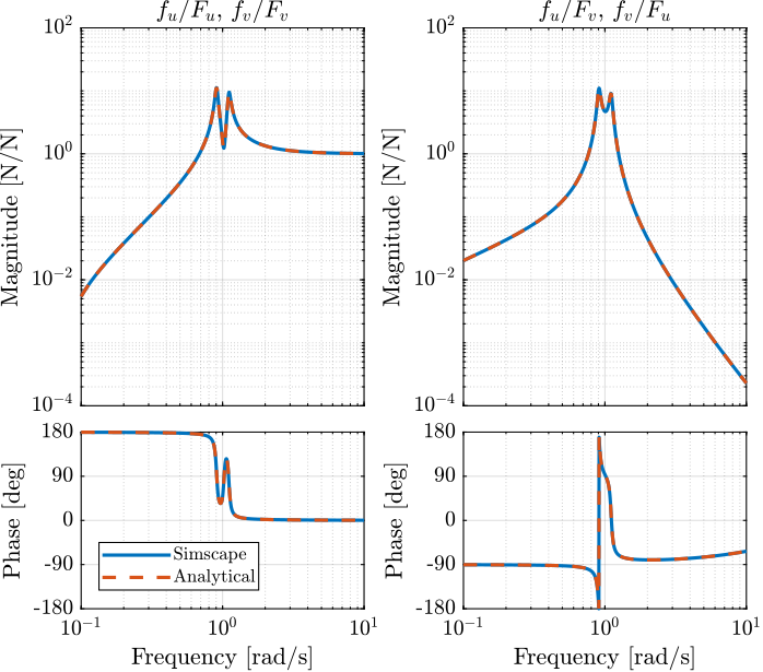
Figure 18: Comparison of the transfer functions from $[F_{u}, F_{v}]$ to $[f_{u}, f_{v}]$ between the Simscape model and the analytical one

4.5 Effect of the parallel stiffness on the IFF plant

The rotation speed is set to $Ω = 0.1 ω_{0}$ .

Copy
  W = 0.1*w0; % [rad/s]

And the IFF plant (transfer function from $[F_{u}, F_{v}]$ to $[f_{u}, f_{v}]$ ) is identified in three different cases:

without parallel stiffness
with a small parallel stiffness $k_{p} < m Ω^{2}$
with a large parallel stiffness $k_{p} > m Ω^{2}$

The results are shown in Figure 19.

One can see that for $k_{p} > m Ω^{2}$ , the systems shows alternating complex conjugate poles and zeros.

Copy  kp = 0;

  w0p = sqrt((k + kp)/m);
  xip = c/(2*sqrt((k+kp)*m));

  Giff = 1/( (s^2/w0p^2 + 2*xip*s/w0p + 1 - W^2/w0p^2)^2 + (2*(s/w0p)*(W/w0p))^2 ) * [ ...
      (s^2/w0p^2 + kp/(k + kp) - W^2/w0p^2)*(s^2/w0p^2 + 2*xip*s/w0p + 1 - W^2/w0p^2) + (2*(s/w0p)*(W/w0p))^2, -(2*xip*s/w0p + k/(k + kp))*(2*(s/w0p)*(W/w0p));
      (2*xip*s/w0p + k/(k + kp))*(2*(s/w0p)*(W/w0p)), (s^2/w0p^2 + kp/(k + kp) - W^2/w0p^2)*(s^2/w0p^2 + 2*xip*s/w0p + 1 - W^2/w0p^2) + (2*(s/w0p)*(W/w0p))^2];

Copy
  kp = 0.5*m*W^2;
  k = 1 - kp;

  w0p = sqrt((k + kp)/m);
  xip = c/(2*sqrt((k+kp)*m));

  Giff_s = 1/( (s^2/w0p^2 + 2*xip*s/w0p + 1 - W^2/w0p^2)^2 + (2*(s/w0p)*(W/w0p))^2 ) * [ ...
      (s^2/w0p^2 + kp/(k + kp) - W^2/w0p^2)*(s^2/w0p^2 + 2*xip*s/w0p + 1 - W^2/w0p^2) + (2*(s/w0p)*(W/w0p))^2, -(2*xip*s/w0p + k/(k + kp))*(2*(s/w0p)*(W/w0p));
      (2*xip*s/w0p + k/(k + kp))*(2*(s/w0p)*(W/w0p)), (s^2/w0p^2 + kp/(k + kp) - W^2/w0p^2)*(s^2/w0p^2 + 2*xip*s/w0p + 1 - W^2/w0p^2) + (2*(s/w0p)*(W/w0p))^2];

Copy
  kp = 1.5*m*W^2;
  k = 1 - kp;

  w0p = sqrt((k + kp)/m);
  xip = c/(2*sqrt((k+kp)*m));

  Giff_l = 1/( (s^2/w0p^2 + 2*xip*s/w0p + 1 - W^2/w0p^2)^2 + (2*(s/w0p)*(W/w0p))^2 ) * [ ...
      (s^2/w0p^2 + kp/(k + kp) - W^2/w0p^2)*(s^2/w0p^2 + 2*xip*s/w0p + 1 - W^2/w0p^2) + (2*(s/w0p)*(W/w0p))^2, -(2*xip*s/w0p + k/(k + kp))*(2*(s/w0p)*(W/w0p));
      (2*xip*s/w0p + k/(k + kp))*(2*(s/w0p)*(W/w0p)), (s^2/w0p^2 + kp/(k + kp) - W^2/w0p^2)*(s^2/w0p^2 + 2*xip*s/w0p + 1 - W^2/w0p^2) + (2*(s/w0p)*(W/w0p))^2];

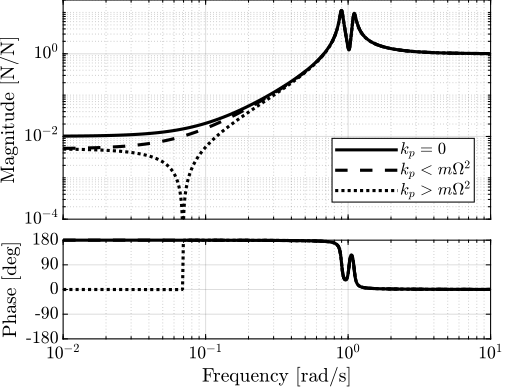
Figure 19: Transfer function from $[F_{u}, F_{v}]$ to $[f_{u}, f_{v}]$ for $k_{p} = 0$ , $k_{p} < m Ω^{2}$ and $k_{p} > m Ω^{2}$

4.6 IFF when adding a spring in parallel

In Figure 20 is displayed the Root Locus in the three considered cases with

\begin{matrix} (23) & K_{IFF} = \frac{g}{s} [\begin{matrix} 1 & 0 \\ 0 & 1 \end{matrix}] \end{matrix}

One can see that for $k_{p} > m Ω^{2}$ , the root locus stays in the left half of the complex plane and thus the control system is unconditionally stable.

Thus, decentralized IFF controller with pure integrators can be used if:

\begin{matrix} (24) & k_{p} > m Ω^{2} \end{matrix}

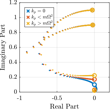
Figure 20: Root Locus

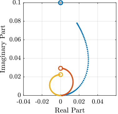
Figure 21: Root Locus

4.7 Effect of $k_{p}$ on the attainable damping

However, having large values of $k_{p}$ may decrease the attainable damping.

To study the second point, Root Locus plots for the following values of $k_{p}$ are shown in Figure 22.

Copy
  kps = [2, 20, 40]*m*W^2;

It is shown that large values of $k_{p}$ decreases the attainable damping.

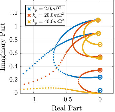
Figure 22: Root Locus plot

Copy
  alphas = logspace(-2, 0, 100);

  opt_xi = zeros(1, length(alphas)); % Optimal simultaneous damping
  opt_gain = zeros(1, length(alphas)); % Corresponding optimal gain

  Kiff = 1/s*eye(2);

  for alpha_i = 1:length(alphas)
      kp = alphas(alpha_i);
      k = 1 - alphas(alpha_i);

      w0p = sqrt((k + kp)/m);
      xip = c/(2*sqrt((k+kp)*m));

      Giff = 1/( (s^2/w0p^2 + 2*xip*s/w0p + 1 - W^2/w0p^2)^2 + (2*(s/w0p)*(W/w0p))^2 ) * [ ...
          (s^2/w0p^2 + kp/(k + kp) - W^2/w0p^2)*(s^2/w0p^2 + 2*xip*s/w0p + 1 - W^2/w0p^2) + (2*(s/w0p)*(W/w0p))^2, -(2*xip*s/w0p + k/(k + kp))*(2*(s/w0p)*(W/w0p));
          (2*xip*s/w0p + k/(k + kp))*(2*(s/w0p)*(W/w0p)), (s^2/w0p^2 + kp/(k + kp) - W^2/w0p^2)*(s^2/w0p^2 + 2*xip*s/w0p + 1 - W^2/w0p^2) + (2*(s/w0p)*(W/w0p))^2];

      fun = @(g)computeSimultaneousDamping(g, Giff, Kiff);

      [g_opt, xi_opt] = fminsearch(fun, 2);
      opt_xi(alpha_i) = 1/xi_opt;
      opt_gain(alpha_i) = g_opt;
  end

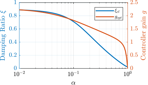
Figure 23: Attainable damping ratio and corresponding controller gain for different parameter $α$

5 Comparison

Two modifications to adapt the IFF control strategy to rotating platforms have been proposed. These two methods are now compared in terms of added damping, closed-loop compliance and transmissibility.

5.1 Plant Parameters

Let’s define initial values for the model.

Copy
  k = 1;    % Actuator Stiffness [N/m]
  c = 0.05; % Actuator Damping [N/(m/s)]
  m = 1;    % Payload mass [kg]

Copy
  xi = c/(2*sqrt(k*m));
  w0 = sqrt(k/m); % [rad/s]

The rotating speed is set to $Ω = 0.1 ω_{0}$ .

Copy
  W = 0.1*w0;

5.2 Root Locus

IFF with High Pass Filter

Copy
  wi = 0.1*w0; % [rad/s]

  Giff = 1/(((s^2)/(w0^2) + 2*xi*s/w0 + 1 - (W^2)/(w0^2))^2 + (2*W*s/(w0^2))^2) * ...
          [(s^2/w0^2 - W^2/w0^2)*((s^2)/(w0^2) + 2*xi*s/w0 + 1 - (W^2)/(w0^2)) + (2*W*s/(w0^2))^2, - (2*xi*s/w0 + 1)*2*W*s/(w0^2) ; ...
           (2*xi*s/w0 + 1)*2*W*s/(w0^2), (s^2/w0^2 - W^2/w0^2)*((s^2)/(w0^2) + 2*xi*s/w0 + 1 - (W^2)/(w0^2))+ (2*W*s/(w0^2))^2];

IFF With parallel Stiffness

Copy
  kp = 5*m*W^2;
  k = k - kp;

  w0p = sqrt((k + kp)/m);
  xip = c/(2*sqrt((k+kp)*m));

  Giff_kp = 1/( (s^2/w0p^2 + 2*xip*s/w0p + 1 - W^2/w0p^2)^2 + (2*(s/w0p)*(W/w0p))^2 ) * [ ...
                     (s^2/w0p^2 + kp/(k + kp) - W^2/w0p^2)*(s^2/w0p^2 + 2*xip*s/w0p + 1 - W^2/w0p^2) + (2*(s/w0p)*(W/w0p))^2, -(2*xip*s/w0p + k/(k + kp))*(2*(s/w0p)*(W/w0p));
                     (2*xip*s/w0p + k/(k + kp))*(2*(s/w0p)*(W/w0p)), (s^2/w0p^2 + kp/(k + kp) - W^2/w0p^2)*(s^2/w0p^2 + 2*xip*s/w0p + 1 - W^2/w0p^2) + (2*(s/w0p)*(W/w0p))^2 ];

  k = k + kp;

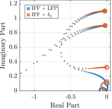
Figure 24: Root Locus plot - Comparison of IFF with additional high pass filter, IFF with additional parallel stiffness

5.3 Controllers - Optimal Gains

In order to compare to three considered Active Damping techniques, gains that yield maximum damping of all the modes are computed for each case.

The obtained damping ratio and control are shown below.

	Obtained $ξ$	Control Gain
Modified IFF	0.83	1.99
IFF with $k_{p}$	0.83	2.02

5.4 Passive Damping - Critical Damping

\begin{matrix} (25) & ξ = \frac{c}{2 \sqrt{k m}} \end{matrix}

Critical Damping corresponds to to $ξ = 1$ , and thus:

\begin{matrix} (26) & c_{crit} = 2 \sqrt{k m} \end{matrix}

Copy
  c_opt = 2*sqrt(k*m);

5.5 Transmissibility And Compliance

Copy
  open('rotating_frame.slx');

Copy
  %% Name of the Simulink File
  mdl = 'rotating_frame';

  %% Input/Output definition
  clear io; io_i = 1;
  io(io_i) = linio([mdl, '/dw'], 1, 'input');  io_i = io_i + 1;
  io(io_i) = linio([mdl, '/fd'], 1, 'input');  io_i = io_i + 1;
  io(io_i) = linio([mdl, '/Meas'], 1, 'output');  io_i = io_i + 1;

Copy  G_ol = linearize(mdl, io, 0);

  %% Input/Output definition
  G_ol.InputName  = {'Dwx', 'Dwy', 'Fdx', 'Fdy'};
  G_ol.OutputName = {'Dx', 'Dy'};

5.5.1 Passive Damping

Copy  kp = 0;
  cp = 0;

Copy  c_old = c;
  c = c_opt;

Copy  G_pas = linearize(mdl, io, 0);

  %% Input/Output definition
  G_pas.InputName  = {'Dwx', 'Dwy', 'Fdx', 'Fdy'};
  G_pas.OutputName = {'Dx', 'Dy'};

Copy  c = c_old;

Copy
  Kiff = opt_gain_iff/(wi + s)*tf(eye(2));

Copy  G_iff = linearize(mdl, io, 0);

  %% Input/Output definition
  G_iff.InputName  = {'Dwx', 'Dwy', 'Fdx', 'Fdy'};
  G_iff.OutputName = {'Dx', 'Dy'};

Copy
  kp = 5*m*W^2;
  cp = 0.01;

Copy
  Kiff = opt_gain_kp/s*tf(eye(2));

Copy  G_kp = linearize(mdl, io, 0);

  %% Input/Output definition
  G_kp.InputName  = {'Dwx', 'Dwy', 'Fdx', 'Fdy'};
  G_kp.OutputName = {'Dx', 'Dy'};

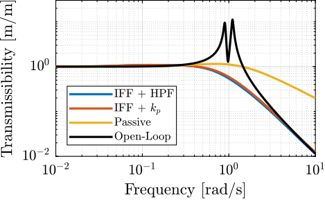
Figure 25: Comparison of the transmissibility

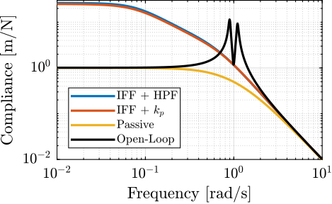
Figure 26: Comparison of the obtained Compliance

6 Notations

	Mathematical Notation	Matlab	Unit
Actuator Stiffness	$k$	`k`	N/m
Actuator Damping	$c$	`c`	N/(m/s)
Payload Mass	$m$	`m`	kg
Damping Ratio	$ξ = \frac{c}{2 \sqrt{k m}}$	`xi`
Actuator Force	$F, F_{u}, F_{v}$	`F` `Fu` `Fv`	N
Force Sensor signal	$f, f_{u}, f_{v}$	`f` `fu` `fv`	N
Relative Displacement	$d, d_{u}, d_{v}$	`d` `du` `dv`	m
Resonance freq. when $Ω = 0$	$ω_{0}$	`w0`	rad/s
Rotation Speed	$Ω = \dot{θ}$	`W`	rad/s
Low Pass Filter corner frequency	$ω_{i}$	`wi`	rad/s

	Mathematical Notation	Matlab	Unit
Laplace variable	$s$	`s`
Complex number	$j$	`j`
Frequency	$ω$	`w`	[rad/s]

Bibliography

Dehaeze, T., and C. Collette. 2020. “Active Damping of Rotating Platforms Using Integral Force Feedback.” In Proceedings of the International Conference on Modal Analysis Noise and Vibration Engineering (ISMA).

Dehaeze, Thomas. 2020. “Active Damping of Rotating Positioning Platforms.” https://doi.org/10.5281/zenodo.3894342.

Dehaeze, Thomas, and Christophe Collette. 2021. “Active Damping of Rotating Platforms Using Integral Force Feedback.” Engineering Research Express. http://iopscience.iop.org/article/10.1088/2631-8695/abe803.

Table of Contents

Active Damping of Rotating Platforms using Integral Force Feedback - Matlab Computation

Table of ContentsClose

1 System Description and Analysis

1.1 System description

1.2 Equations

1.3 Numerical Values

1.4 Campbell Diagram

1.5 Simscape Model

1.6 Effect of the rotation speed

2 Problem with pure Integral Force Feedback

2.1 Plant Parameters

2.2 Equations

2.3 Comparison of the Analytical Model and the Simscape Model

2.4 Effect of the rotation speed

2.5 Decentralized Integral Force Feedback

3 Integral Force Feedback with an High Pass Filter

3.1 Plant Parameters

3.2 Modified Integral Force Feedback Controller

3.3 Root Locus

3.4 What is the optimal ωi and g?

4 IFF with a stiffness in parallel with the force sensor

4.1 Schematic

4.2 Equations

4.3 Plant Parameters

4.4 Comparison of the Analytical Model and the Simscape Model

4.5 Effect of the parallel stiffness on the IFF plant

4.6 IFF when adding a spring in parallel

4.7 Effect of kp on the attainable damping

5 Comparison

5.1 Plant Parameters

5.2 Root Locus

5.3 Controllers - Optimal Gains

5.4 Passive Damping - Critical Damping

5.5 Transmissibility And Compliance

5.5.1 Passive Damping

6 Notations

Bibliography

3.4 What is the optimal $ω_{i}$ and $g$ ?

4.7 Effect of $k_{p}$ on the attainable damping