Complementary Filters Shaping Using \(\mathcal{H}_\infty\) Synthesis - Matlab Computation
Table of Contents
In this document, the design of complementary filters is studied.
One use of complementary filter is described below:
The basic idea of a complementary filter involves taking two or more sensors, filtering out unreliable frequencies for each sensor, and combining the filtered outputs to get a better estimate throughout the entire bandwidth of the system. To achieve this, the sensors included in the filter should complement one another by performing better over specific parts of the system bandwidth.
- in section 1, the \(\mathcal{H}_\infty\) synthesis is used for generating two complementary filters
- in section 2, a method using the \(\mathcal{H}_\infty\) synthesis is proposed to shape three of more complementary filters
- in section 3, the \(\mathcal{H}_\infty\) synthesis is used and compared with FIR complementary filters used for LIGO
Add the Matlab code use to obtain the results presented in the paper are accessible here and presented below.
1 H-Infinity synthesis of complementary filters
The Matlab file corresponding to this section is accessible here.
1.1 Synthesis Architecture
We here synthesize two complementary filters using the \(\mathcal{H}_\infty\) synthesis. The goal is to specify upper bounds on the norms of the two complementary filters \(H_1(s)\) and \(H_2(s)\) while ensuring their complementary property (\(H_1(s) + H_2(s) = 1\)).
In order to do so, we use the generalized plant shown on figure 1 where \(W_1(s)\) and \(W_2(s)\) are weighting transfer functions that will be used to shape \(H_1(s)\) and \(H_2(s)\) respectively.
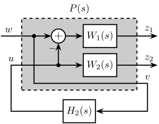
Figure 1: \(\mathcal{H}_\infty\) synthesis of the complementary filters
The \(\mathcal{H}_\infty\) synthesis applied on this generalized plant will give a transfer function \(H_2\) (figure 1) such that the \(\mathcal{H}_\infty\) norm of the transfer function from \(w\) to \([z_1,\ z_2]\) is less than one: \[ \left\| \begin{array}{c} (1 - H_2(s)) W_1(s) \\ H_2(s) W_2(s) \end{array} \right\|_\infty < 1 \]
Thus, if the above condition is verified, we can define \(H_1(s) = 1 - H_2(s)\) and we have that: \[ \left\| \begin{array}{c} H_1(s) W_1(s) \\ H_2(s) W_2(s) \end{array} \right\|_\infty < 1 \] Which is almost (with an maximum error of \(\sqrt{2}\)) equivalent to:
\begin{align*} |H_1(j\omega)| &< \frac{1}{|W_1(j\omega)|}, \quad \forall \omega \\ |H_2(j\omega)| &< \frac{1}{|W_2(j\omega)|}, \quad \forall \omega \end{align*}We then see that \(W_1(s)\) and \(W_2(s)\) can be used to shape both \(H_1(s)\) and \(H_2(s)\) while ensuring their complementary property by the definition of \(H_1(s) = 1 - H_2(s)\).
1.2 Design of Weighting Function
A formula is proposed to help the design of the weighting functions:
\begin{equation} W(s) = \left( \frac{ \frac{1}{\omega_0} \sqrt{\frac{1 - \left(\frac{G_0}{G_c}\right)^{\frac{2}{n}}}{1 - \left(\frac{G_c}{G_\infty}\right)^{\frac{2}{n}}}} s + \left(\frac{G_0}{G_c}\right)^{\frac{1}{n}} }{ \left(\frac{1}{G_\infty}\right)^{\frac{1}{n}} \frac{1}{\omega_0} \sqrt{\frac{1 - \left(\frac{G_0}{G_c}\right)^{\frac{2}{n}}}{1 - \left(\frac{G_c}{G_\infty}\right)^{\frac{2}{n}}}} s + \left(\frac{1}{G_c}\right)^{\frac{1}{n}} }\right)^n \end{equation}The parameters permits to specify:
- the low frequency gain: \(G_0 = lim_{\omega \to 0} |W(j\omega)|\)
- the high frequency gain: \(G_\infty = lim_{\omega \to \infty} |W(j\omega)|\)
- the absolute gain at \(\omega_0\): \(G_c = |W(j\omega_0)|\)
- the absolute slope between high and low frequency: \(n\)
The general shape of a weighting function generated using the formula is shown in figure 2.
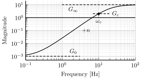
Figure 2: Amplitude of the proposed formula for the weighting functions
n = 2; w0 = 2*pi*11; G0 = 1/10; G1 = 1000; Gc = 1/2;
W1 = (((1/w0)*sqrt((1-(G0/Gc)^(2/n))/(1-(Gc/G1)^(2/n)))*s + (G0/Gc)^(1/n))/((1/G1)^(1/n)*(1/w0)*sqrt((1-(G0/Gc)^(2/n))/(1-(Gc/G1)^(2/n)))*s + (1/Gc)^(1/n)))^n;

n = 3; w0 = 2*pi*10; G0 = 1000; G1 = 0.1; Gc = 1/2;
W2 = (((1/w0)*sqrt((1-(G0/Gc)^(2/n))/(1-(Gc/G1)^(2/n)))*s + (G0/Gc)^(1/n))/((1/G1)^(1/n)*(1/w0)*sqrt((1-(G0/Gc)^(2/n))/(1-(Gc/G1)^(2/n)))*s + (1/Gc)^(1/n)))^n;

Figure 3: Weights on the complementary filters \(W_1\) and \(W_2\) and the associated performance weights
1.3 H-Infinity Synthesis
We define the generalized plant \(P\) on matlab.
P = [W1 -W1;
     0   W2;
     1   0];
And we do the \(\mathcal{H}_\infty\) synthesis using the hinfsyn command.
[H2, ~, gamma, ~] = hinfsyn(P, 1, 1,'TOLGAM', 0.001, 'METHOD', 'ric', 'DISPLAY', 'on');
[H2, ~, gamma, ~] = hinfsyn(P, 1, 1,'TOLGAM', 0.001, 'METHOD', 'ric', 'DISPLAY', 'on');
Resetting value of Gamma min based on D_11, D_12, D_21 terms

Test bounds:      0.1000 <  gamma  <=   1050.0000

  gamma    hamx_eig  xinf_eig  hamy_eig   yinf_eig   nrho_xy   p/f
1.050e+03   2.8e+01   2.4e-07   4.1e+00    0.0e+00    0.0000    p
  525.050   2.8e+01   2.4e-07   4.1e+00    0.0e+00    0.0000    p
  262.575   2.8e+01   2.4e-07   4.1e+00    0.0e+00    0.0000    p
  131.337   2.8e+01   2.4e-07   4.1e+00   -1.0e-13    0.0000    p
   65.719   2.8e+01   2.4e-07   4.1e+00   -9.5e-14    0.0000    p
   32.909   2.8e+01   2.4e-07   4.1e+00    0.0e+00    0.0000    p
   16.505   2.8e+01   2.4e-07   4.1e+00   -1.0e-13    0.0000    p
    8.302   2.8e+01   2.4e-07   4.1e+00   -7.2e-14    0.0000    p
    4.201   2.8e+01   2.4e-07   4.1e+00   -2.5e-25    0.0000    p
    2.151   2.7e+01   2.4e-07   4.1e+00   -3.8e-14    0.0000    p
    1.125   2.6e+01   2.4e-07   4.1e+00   -5.4e-24    0.0000    p
    0.613   2.3e+01 -3.7e+01#  4.1e+00    0.0e+00    0.0000    f
    0.869   2.6e+01 -3.7e+02#  4.1e+00    0.0e+00    0.0000    f
    0.997   2.6e+01 -1.1e+04#  4.1e+00    0.0e+00    0.0000    f
    1.061   2.6e+01   2.4e-07   4.1e+00    0.0e+00    0.0000    p
    1.029   2.6e+01   2.4e-07   4.1e+00    0.0e+00    0.0000    p
    1.013   2.6e+01   2.4e-07   4.1e+00    0.0e+00    0.0000    p
    1.005   2.6e+01   2.4e-07   4.1e+00    0.0e+00    0.0000    p
    1.001   2.6e+01 -3.1e+04#  4.1e+00   -3.8e-14    0.0000    f
    1.003   2.6e+01 -2.8e+05#  4.1e+00    0.0e+00    0.0000    f
    1.004   2.6e+01   2.4e-07   4.1e+00   -5.8e-24    0.0000    p
    1.004   2.6e+01   2.4e-07   4.1e+00    0.0e+00    0.0000    p

 Gamma value achieved:     1.0036
We then define the high pass filter \(H_1 = 1 - H_2\). The bode plot of both \(H_1\) and \(H_2\) is shown on figure 4.
H1 = 1 - H2;
1.4 Obtained Complementary Filters
The obtained complementary filters are shown on figure 4.
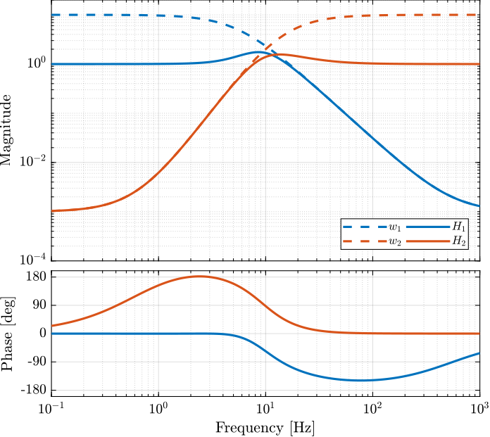
Figure 4: Obtained complementary filters using \(\mathcal{H}_\infty\) synthesis
2 Generating 3 complementary filters
The Matlab file corresponding to this section is accessible here.
2.1 Theory
We want:
\begin{align*} & |H_1(j\omega)| < 1/|W_1(j\omega)|, \quad \forall\omega\\ & |H_2(j\omega)| < 1/|W_2(j\omega)|, \quad \forall\omega\\ & |H_3(j\omega)| < 1/|W_3(j\omega)|, \quad \forall\omega\\ & H_1(s) + H_2(s) + H_3(s) = 1 \end{align*}For that, we use the \(\mathcal{H}_\infty\) synthesis with the architecture shown on figure 5.
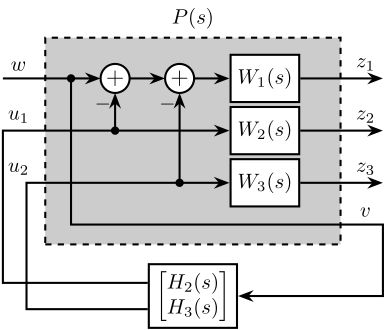
Figure 5: Generalized architecture for generating 3 complementary filters
The \(\mathcal{H}_\infty\) objective is:
\begin{align*} & |(1 - H_2(j\omega) - H_3(j\omega)) W_1(j\omega)| < 1, \quad \forall\omega\\ & |H_2(j\omega) W_2(j\omega)| < 1, \quad \forall\omega\\ & |H_3(j\omega) W_3(j\omega)| < 1, \quad \forall\omega\\ \end{align*}And thus if we choose \(H_1 = 1 - H_2 - H_3\) we have solved the problem.
2.2 Weights
First we define the weights.
n = 2; w0 = 2*pi*1; G0 = 1/10; G1 = 1000; Gc = 1/2;
W1 = (((1/w0)*sqrt((1-(G0/Gc)^(2/n))/(1-(Gc/G1)^(2/n)))*s + (G0/Gc)^(1/n))/((1/G1)^(1/n)*(1/w0)*sqrt((1-(G0/Gc)^(2/n))/(1-(Gc/G1)^(2/n)))*s + (1/Gc)^(1/n)))^n;

W2 = 0.22*(1 + s/2/pi/1)^2/(sqrt(1e-4) + s/2/pi/1)^2*(1 + s/2/pi/10)^2/(1 + s/2/pi/1000)^2;

n = 3; w0 = 2*pi*10; G0 = 1000; G1 = 0.1; Gc = 1/2;
W3 = (((1/w0)*sqrt((1-(G0/Gc)^(2/n))/(1-(Gc/G1)^(2/n)))*s + (G0/Gc)^(1/n))/((1/G1)^(1/n)*(1/w0)*sqrt((1-(G0/Gc)^(2/n))/(1-(Gc/G1)^(2/n)))*s + (1/Gc)^(1/n)))^n;
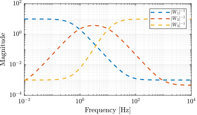
Figure 6: Three weighting functions used for the \(\mathcal{H}_\infty\) synthesis of the complementary filters
2.3 H-Infinity Synthesis
Then we create the generalized plant P.
P = [W1 -W1 -W1;
     0   W2  0 ;
     0   0   W3;
     1   0   0];
And we do the \(\mathcal{H}_\infty\) synthesis.
[H, ~, gamma, ~] = hinfsyn(P, 1, 2,'TOLGAM', 0.001, 'METHOD', 'ric', 'DISPLAY', 'on');
[H, ~, gamma, ~] = hinfsyn(P, 1, 2,'TOLGAM', 0.001, 'METHOD', 'ric', 'DISPLAY', 'on');
Resetting value of Gamma min based on D_11, D_12, D_21 terms

Test bounds:      0.1000 <  gamma  <=   1050.0000

  gamma    hamx_eig  xinf_eig  hamy_eig   yinf_eig   nrho_xy   p/f
1.050e+03   3.2e+00   4.5e-13   6.3e-02   -1.2e-11    0.0000    p
  525.050   3.2e+00   1.3e-13   6.3e-02    0.0e+00    0.0000    p
  262.575   3.2e+00   2.1e-12   6.3e-02   -1.5e-13    0.0000    p
  131.337   3.2e+00   1.1e-12   6.3e-02   -7.2e-29    0.0000    p
   65.719   3.2e+00   2.0e-12   6.3e-02    0.0e+00    0.0000    p
   32.909   3.2e+00   7.4e-13   6.3e-02   -5.9e-13    0.0000    p
   16.505   3.2e+00   1.4e-12   6.3e-02    0.0e+00    0.0000    p
    8.302   3.2e+00   1.6e-12   6.3e-02    0.0e+00    0.0000    p
    4.201   3.2e+00   1.6e-12   6.3e-02    0.0e+00    0.0000    p
    2.151   3.2e+00   1.6e-12   6.3e-02    0.0e+00    0.0000    p
    1.125   3.2e+00   2.8e-12   6.3e-02    0.0e+00    0.0000    p
    0.613   3.0e+00 -2.5e+03#  6.3e-02    0.0e+00    0.0000    f
    0.869   3.1e+00 -2.9e+01#  6.3e-02    0.0e+00    0.0000    f
    0.997   3.2e+00   1.9e-12   6.3e-02    0.0e+00    0.0000    p
    0.933   3.1e+00 -6.9e+02#  6.3e-02    0.0e+00    0.0000    f
    0.965   3.1e+00 -3.0e+03#  6.3e-02    0.0e+00    0.0000    f
    0.981   3.1e+00 -8.6e+03#  6.3e-02    0.0e+00    0.0000    f
    0.989   3.2e+00 -2.7e+04#  6.3e-02    0.0e+00    0.0000    f
    0.993   3.2e+00 -5.7e+05#  6.3e-02    0.0e+00    0.0000    f
    0.995   3.2e+00   2.2e-12   6.3e-02    0.0e+00    0.0000    p
    0.994   3.2e+00   1.6e-12   6.3e-02    0.0e+00    0.0000    p
    0.994   3.2e+00   1.0e-12   6.3e-02    0.0e+00    0.0000    p

 Gamma value achieved:     0.9936
2.4 Obtained Complementary Filters
The obtained filters are:
H2 = tf(H(1));
H3 = tf(H(2));
H1 = 1 - H2 - H3;
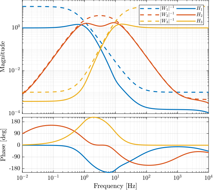
Figure 7: The three complementary filters obtained after \(\mathcal{H}_\infty\) synthesis
3 Try to implement complementary filters for LIGO
The Matlab file corresponding to this section is accessible here.
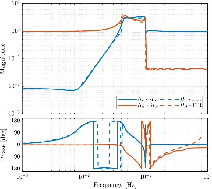
Let’s try to design complementary filters that are corresponding to the complementary filters design for the LIGO and described in (Hua 2005).
The FIR complementary filters designed in (Hua 2005) are of order 512.
3.1 Specifications
The specifications for the filters are:
- From \(0\) to \(0.008\text{ Hz}\),the magnitude of the filter’s transfer function should be less than or equal to \(8 \times 10^{-3}\)
- From \(0.008\text{ Hz}\) to \(0.04\text{ Hz}\), it attenuates the input signal proportional to frequency cubed
- Between \(0.04\text{ Hz}\) and \(0.1\text{ Hz}\), the magnitude of the transfer function should be less than 3
- Above \(0.1\text{ Hz}\), the maximum of the magnitude of the complement filter should be as close to zero as possible. In our system, we would like to have the magnitude of the complementary filter to be less than \(0.1\). As the filters obtained in (Hua 2005) have a magnitude of \(0.045\), we will set that as our requirement
The specifications are translated in upper bounds of the complementary filters are shown on figure 8.
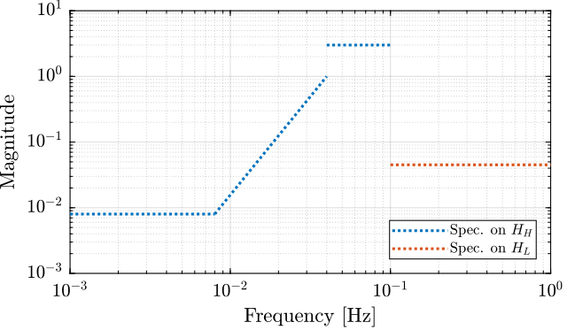
Figure 8: Specification for the LIGO complementary filters
3.2 FIR Filter
We here try to implement the FIR complementary filter synthesis as explained in (Hua 2005). For that, we use the CVX matlab Toolbox.
We setup the CVX toolbox and use the SeDuMi solver.
cvx_startup;
cvx_solver sedumi;
We define the frequency vectors on which we will constrain the norm of the FIR filter.
w1 = 0:4.06e-4:0.008;
w2 = 0.008:4.06e-4:0.04;
w3 = 0.04:8.12e-4:0.1;
w4 = 0.1:8.12e-4:0.83;
We then define the order of the FIR filter.
n = 512;
A1 = [ones(length(w1),1),  cos(kron(w1'.*(2*pi),[1:n-1]))];
A2 = [ones(length(w2),1),  cos(kron(w2'.*(2*pi),[1:n-1]))];
A3 = [ones(length(w3),1),  cos(kron(w3'.*(2*pi),[1:n-1]))];
A4 = [ones(length(w4),1),  cos(kron(w4'.*(2*pi),[1:n-1]))];

B1 = [zeros(length(w1),1), sin(kron(w1'.*(2*pi),[1:n-1]))];
B2 = [zeros(length(w2),1), sin(kron(w2'.*(2*pi),[1:n-1]))];
B3 = [zeros(length(w3),1), sin(kron(w3'.*(2*pi),[1:n-1]))];
B4 = [zeros(length(w4),1), sin(kron(w4'.*(2*pi),[1:n-1]))];
We run the convex optimization.
cvx_begin

variable y(n+1,1)

% t
maximize(-y(1))

for i = 1:length(w1)
    norm([0 A1(i,:); 0 B1(i,:)]*y) <= 8e-3;
end

for  i = 1:length(w2)
    norm([0 A2(i,:); 0 B2(i,:)]*y) <= 8e-3*(2*pi*w2(i)/(0.008*2*pi))^3;
end

for i = 1:length(w3)
    norm([0 A3(i,:); 0 B3(i,:)]*y) <= 3;
end

for i = 1:length(w4)
    norm([[1 0]'- [0 A4(i,:); 0 B4(i,:)]*y]) <= y(1);
end

cvx_end

h = y(2:end);
cvx_begin
variable y(n+1,1)
% t
maximize(-y(1))
for i = 1:length(w1)
    norm([0 A1(i,:); 0 B1(i,:)]*y) <= 8e-3;
end
for  i = 1:length(w2)
    norm([0 A2(i,:); 0 B2(i,:)]*y) <= 8e-3*(2*pi*w2(i)/(0.008*2*pi))^3;
end
for i = 1:length(w3)
    norm([0 A3(i,:); 0 B3(i,:)]*y) <= 3;
end
for i = 1:length(w4)
    norm([[1 0]'- [0 A4(i,:); 0 B4(i,:)]*y]) <= y(1);
end
cvx_end

Calling SeDuMi 1.34: 4291 variables, 1586 equality constraints
   For improved efficiency, SeDuMi is solving the dual problem.
------------------------------------------------------------
SeDuMi 1.34 (beta) by AdvOL, 2005-2008 and Jos F. Sturm, 1998-2003.
Alg = 2: xz-corrector, Adaptive Step-Differentiation, theta = 0.250, beta = 0.500
eqs m = 1586, order n = 3220, dim = 4292, blocks = 1073
nnz(A) = 1100727 + 0, nnz(ADA) = 1364794, nnz(L) = 683190
 it :     b*y       gap    delta  rate   t/tP*  t/tD*   feas cg cg  prec
  0 :            4.11E+02 0.000
  1 :  -2.58E+00 1.25E+02 0.000 0.3049 0.9000 0.9000   4.87  1  1  3.0E+02
  2 :  -2.36E+00 3.90E+01 0.000 0.3118 0.9000 0.9000   1.83  1  1  6.6E+01
  3 :  -1.69E+00 1.31E+01 0.000 0.3354 0.9000 0.9000   1.76  1  1  1.5E+01
  4 :  -8.60E-01 7.10E+00 0.000 0.5424 0.9000 0.9000   2.48  1  1  4.8E+00
  5 :  -4.91E-01 5.44E+00 0.000 0.7661 0.9000 0.9000   3.12  1  1  2.5E+00
  6 :  -2.96E-01 3.88E+00 0.000 0.7140 0.9000 0.9000   2.62  1  1  1.4E+00
  7 :  -1.98E-01 2.82E+00 0.000 0.7271 0.9000 0.9000   2.14  1  1  8.5E-01
  8 :  -1.39E-01 2.00E+00 0.000 0.7092 0.9000 0.9000   1.78  1  1  5.4E-01
  9 :  -9.99E-02 1.30E+00 0.000 0.6494 0.9000 0.9000   1.51  1  1  3.3E-01
 10 :  -7.57E-02 8.03E-01 0.000 0.6175 0.9000 0.9000   1.31  1  1  2.0E-01
 11 :  -5.99E-02 4.22E-01 0.000 0.5257 0.9000 0.9000   1.17  1  1  1.0E-01
 12 :  -5.28E-02 2.45E-01 0.000 0.5808 0.9000 0.9000   1.08  1  1  5.9E-02
 13 :  -4.82E-02 1.28E-01 0.000 0.5218 0.9000 0.9000   1.05  1  1  3.1E-02
 14 :  -4.56E-02 5.65E-02 0.000 0.4417 0.9045 0.9000   1.02  1  1  1.4E-02
 15 :  -4.43E-02 2.41E-02 0.000 0.4265 0.9004 0.9000   1.01  1  1  6.0E-03
 16 :  -4.37E-02 8.90E-03 0.000 0.3690 0.9070 0.9000   1.00  1  1  2.3E-03
 17 :  -4.35E-02 3.24E-03 0.000 0.3641 0.9164 0.9000   1.00  1  1  9.5E-04
 18 :  -4.34E-02 1.55E-03 0.000 0.4788 0.9086 0.9000   1.00  1  1  4.7E-04
 19 :  -4.34E-02 8.77E-04 0.000 0.5653 0.9169 0.9000   1.00  1  1  2.8E-04
 20 :  -4.34E-02 5.05E-04 0.000 0.5754 0.9034 0.9000   1.00  1  1  1.6E-04
 21 :  -4.34E-02 2.94E-04 0.000 0.5829 0.9136 0.9000   1.00  1  1  9.9E-05
 22 :  -4.34E-02 1.63E-04 0.015 0.5548 0.9000 0.0000   1.00  1  1  6.6E-05
 23 :  -4.33E-02 9.42E-05 0.000 0.5774 0.9053 0.9000   1.00  1  1  3.9E-05
 24 :  -4.33E-02 6.27E-05 0.000 0.6658 0.9148 0.9000   1.00  1  1  2.6E-05
 25 :  -4.33E-02 3.75E-05 0.000 0.5972 0.9187 0.9000   1.00  1  1  1.6E-05
 26 :  -4.33E-02 1.89E-05 0.000 0.5041 0.9117 0.9000   1.00  1  1  8.6E-06
 27 :  -4.33E-02 9.72E-06 0.000 0.5149 0.9050 0.9000   1.00  1  1  4.5E-06
 28 :  -4.33E-02 2.94E-06 0.000 0.3021 0.9194 0.9000   1.00  1  1  1.5E-06
 29 :  -4.33E-02 9.73E-07 0.000 0.3312 0.9189 0.9000   1.00  2  2  5.3E-07
 30 :  -4.33E-02 2.82E-07 0.000 0.2895 0.9063 0.9000   1.00  2  2  1.6E-07
 31 :  -4.33E-02 8.05E-08 0.000 0.2859 0.9049 0.9000   1.00  2  2  4.7E-08
 32 :  -4.33E-02 1.43E-08 0.000 0.1772 0.9059 0.9000   1.00  2  2  8.8E-09

iter seconds digits       c*x               b*y
 32     49.4   6.8 -4.3334083581e-02 -4.3334090214e-02
|Ax-b| =   3.7e-09, [Ay-c]_+ =   1.1E-10, |x|=  1.0e+00, |y|=  2.6e+00

Detailed timing (sec)
   Pre          IPM          Post
3.902E+00    4.576E+01    1.035E-02
Max-norms: ||b||=1, ||c|| = 3,
Cholesky |add|=0, |skip| = 0, ||L.L|| = 4.26267.
------------------------------------------------------------
Status: Solved
Optimal value (cvx_optval): -0.0433341
h = y(2:end);
Finally, we compute the filter response over the frequency vector defined and the result is shown on figure 9 which is very close to the filters obtain in (Hua 2005).
w = [w1 w2 w3 w4];
H = [exp(-j*kron(w'.*2*pi,[0:n-1]))]*h;
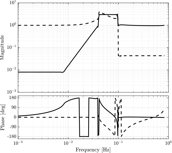
Figure 9: FIR Complementary filters obtain after convex optimization
3.3 Weights
We design weights that will be used for the \(\mathcal{H}_\infty\) synthesis of the complementary filters. These weights will determine the order of the obtained filters. Here are the requirements on the filters:
- reasonable order
- to be as close as possible to the specified upper bounds
- stable minimum phase
The bode plot of the weights is shown on figure 10.
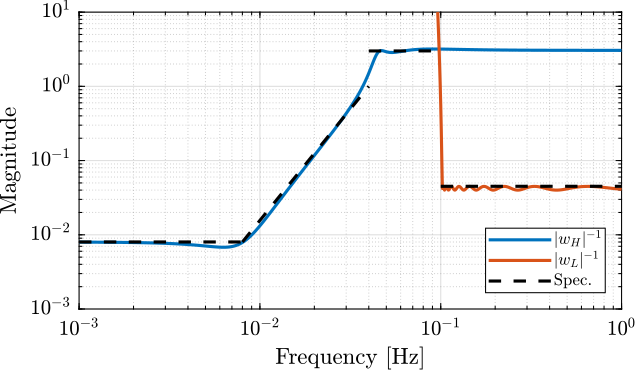
Figure 10: Weights for the \(\mathcal{H}_\infty\) synthesis
3.4 H-Infinity Synthesis
We define the generalized plant as shown on figure 1.
P = [0   wL;
     wH -wH;
     1   0];
And we do the \(\mathcal{H}_\infty\) synthesis using the hinfsyn command.
[Hl, ~, gamma, ~] = hinfsyn(P, 1, 1,'TOLGAM', 0.001, 'METHOD', 'ric', 'DISPLAY', 'on');
[Hl, ~, gamma, ~] = hinfsyn(P, 1, 1,'TOLGAM', 0.001, 'METHOD', 'ric', 'DISPLAY', 'on');
Resetting value of Gamma min based on D_11, D_12, D_21 terms

Test bounds:      0.3276 <  gamma  <=      1.8063

  gamma    hamx_eig  xinf_eig  hamy_eig   yinf_eig   nrho_xy   p/f
    1.806   1.4e-02 -1.7e-16   3.6e-03   -4.8e-12    0.0000    p
    1.067   1.3e-02 -4.2e-14   3.6e-03   -1.9e-12    0.0000    p
    0.697   1.3e-02 -3.0e-01#  3.6e-03   -3.5e-11    0.0000    f
    0.882   1.3e-02 -9.5e-01#  3.6e-03   -1.2e-34    0.0000    f
    0.975   1.3e-02 -2.7e+00#  3.6e-03   -1.6e-12    0.0000    f
    1.021   1.3e-02 -8.7e+00#  3.6e-03   -4.5e-16    0.0000    f
    1.044   1.3e-02 -6.5e-14   3.6e-03   -3.0e-15    0.0000    p
    1.032   1.3e-02 -1.8e+01#  3.6e-03    0.0e+00    0.0000    f
    1.038   1.3e-02 -3.8e+01#  3.6e-03    0.0e+00    0.0000    f
    1.041   1.3e-02 -8.3e+01#  3.6e-03   -2.9e-33    0.0000    f
    1.042   1.3e-02 -1.9e+02#  3.6e-03   -3.4e-11    0.0000    f
    1.043   1.3e-02 -5.3e+02#  3.6e-03   -7.5e-13    0.0000    f

 Gamma value achieved:     1.0439
The high pass filter is defined as \(H_H = 1 - H_L\).
Hh = 1 - Hl;
The size of the filters is shown below.
State-space model with 1 outputs, 1 inputs, and 27 states.
State-space model with 1 outputs, 1 inputs, and 27 states.
The bode plot of the obtained filters as shown on figure 11.
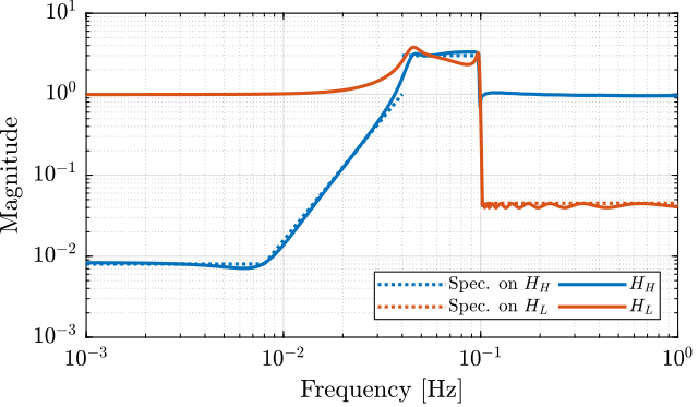
Figure 11: Obtained complementary filters using the \(\mathcal{H}_\infty\) synthesis