DCM - Laser Setup

1. Experimental Setup
2. Alignment of metrology
3. Photo-diodes Calibration
4. Noise Measurement
5. Noise budgeting
6. Stability Measurement

This report is also available as a pdf.

The “Laser Setup” is used for the commissioning of the ESRF Double Crystal Monochromator (DCM). More precisely, it is used to measure the output beam position errors.

This document is structured as follow:

Section 1: the experimental setup is described
Section 2: the alignment of the metrology is performed
Section 3: the quadrant photodiodes are calibrated
Section 4: the high frequency (i.e. above 1Hz) noise is measured and the limitations are identified
Section 6: the low frequency drifts are measured and solution to limit these drifts are proposed and tested

1. Experimental Setup

1.1. Specifications

The goal of the Laser Setup is to measure the motion errors of the DCM. Specifications in terms of DCM’s second crystal movements are summarized in Table 1. As shown, three position variables are important for the DCM that corresponds to a default of parallelism between the crystal (dRx and dRy) and to a default of distance between the crystals (dDz).

Table 1: Specification in terms of measured DCM relative crystal motion
Motion	Range	Stability (5 min)	Noise (200Hz BW)
`dRx`	50 urad	100 nrad	20 nrad RMS
`dRy`	50 urad	50 nrad	10 nrad RMS
`dDz`	10 um		100 nm RMS

These defaults will be transmitted to angular and position motion of the output beam.

In order to measure the DCM positioning defaults, the output beam pose, defined by four degrees of freedom (Dy, Dz, Dy and Rz), has to be measured. The specification of the beam pose metrology are specified in Table 2.

Table 2: Specification in terms of measured beam pose
Motion	Range	Stability (5 min)	Noise (200Hz BW)
`Rx`	100 urad	200 nrad	40 nrad RMS
`Ry`	100 urad	100 nrad	20 nrad RMS
`Dz`	10 um
`Dy`	-	-	-

Note the factor two between Table 1 and Table 2. This is due to the fact that an angular motion of dRx or dRy will induce twice the motion of the output beam angle.

Moreover, the measurement bandwidth should be higher than 1 kHz.

1.2. Optical Schematic

A simplified optical schematic of the laser setup is shown in Figure 1.

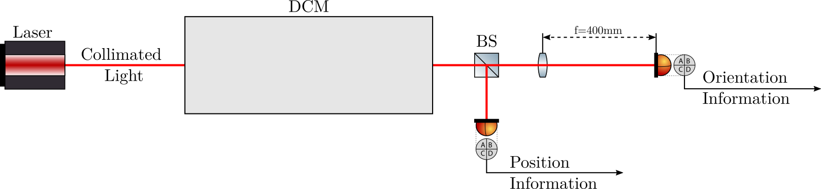
Figure 1: Schematic of the optical setup

The Diameter of the laser beam is 4mm (\(1/e^2\)). A 50/50 beam splitter (BS) is used to separate the incoming beam in two. One part is used to measured the translation of the beam using one quadrant photodiode.

The other part is used to measured angular motion of the beam. To do so, a Lens with focal of 400mm is used, and the quadrant photodiode is positioned at the focal plane of the lens (see Figure 2). In such a case, the position of the focused beam on the quadrant photodiode depends only of the angle of the incoming beam and not of its position.

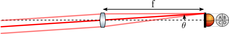
Figure 2: Working principle of a lens and a quadrant photodiode at its focal plane

1.3. Instrumentation

1.3.1. Four Quadrant Photodiode

Two identical quadrant photodiodes are used as explained in Section 1.2. These photodiodes are visually shown in Figure 3 and their spectral response in Figure 4.

Table 3: Characteristics of the Four Quadrant Photodiode (doc)
Characteristic	Value
Gap	\(18\,\mu m\)
Capacitance	\(25\,pF\)

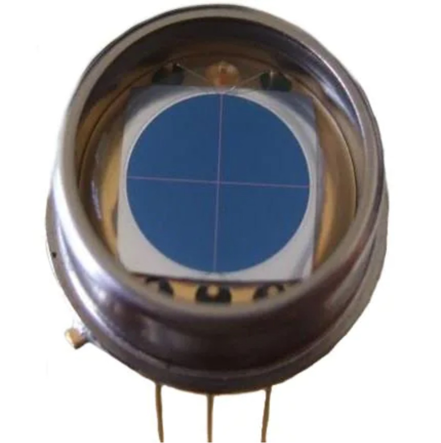
Figure 3: Picture of the Four Quadrant Photodiode

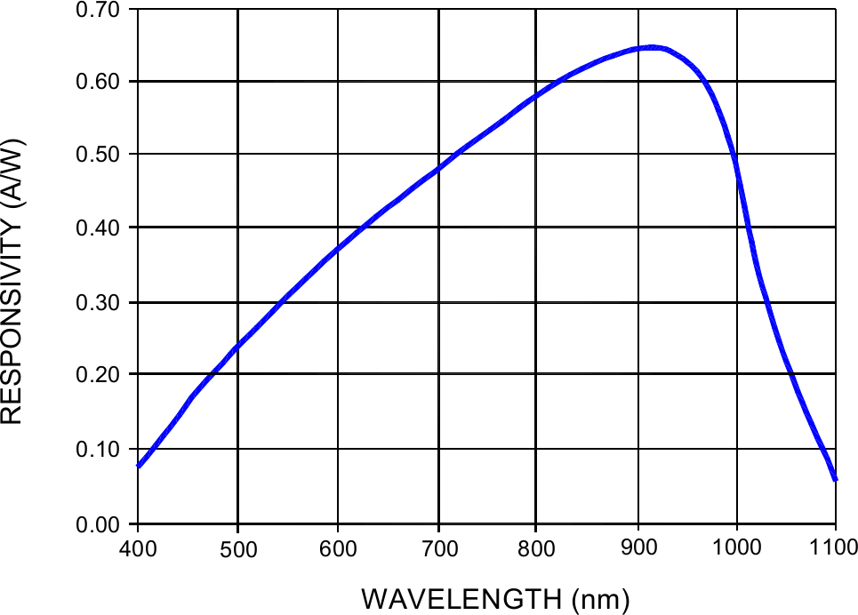
Figure 4: Spectral Response of the Four Quadrant Photodiode

1.3.2. Transimpedance Amplifier

In order to measure the generated current on each quadrant of the photodiodes, transimpedance amplifiers are used.

The characteristics of the amplifiers are summarized in Table 4.

Table 4: Characteristics of the transimpedance amplifier (doc)
Characteristic	Value
Bandwidth (3dB)	\(100\,kHz\)
Gain	\(100\,kV/A\)
Input Current Noise	\(0.36\,pA/\sqrt{Hz}\)
Output Voltage Range	-2V to 2V

The expected amplitude spectral density of the amplifier’s output voltage noise is:

\begin{equation} \Gamma_{V} = R_f \cdot \Gamma_{I} \end{equation}

with \(\Gamma_V\) the output voltage noise ASD in \(V/\sqrt{Hz}\), \(\Gamma_I\) the input current noise ASD in \(A/\sqrt{Hz}\), and \(R_f\) is the transimpedance amplifier gain in \(V/A\).

We obtain:

\begin{equation} \boxed{\Gamma_V \approx 3.6 \cdot 10^{-8}\, V/\sqrt{Hz}} \end{equation}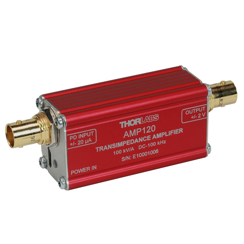

Figure 5: Picture of the transimpedance amplifier

The amplifier noise is most probably dominated by the “Johnson noise” which is flat with frequency and equal to (see (Horowitz 2015), chapter 8.11):

\begin{equation} \Gamma_I = \sqrt{4 k T/R_f} \end{equation}

with \(k = 1.38 \cdot 10^{-23}\,\text{joules/K}\) the Boltzman’s constant, \(T\) is the absolute temperature in Kelvin, and \(R_f\) is the transimpedance amplifier gain in \(\Omega = V/A\).

At \(T = 20^oC\), we obtain \(\Gamma_I \approx 0.4\,pA/\sqrt{Hz}\) which is very close to the input current noise amplitude spectral density specified in the documentation.

1.3.3. Analog to Digital Converters

The output voltage of the transimpedance amplifiers are digitized using Analog to Digital converters (ADC).

The ADC used are from the Speedgoat IO131 or IO322 boards. Their characteristics are summarized in Table 5.

Table 5: Characteristics of the Analog to Digital Converters (doc)
Characteristic	Value
Input Range	\(\pm 10.24\,V\) \(\pm 5.12\,V\) \(\pm 2.56\,V\) \(\pm 1.28\,V\)
Accuracy	\(0.015\,\%\) (\(\pm 2.56\,V\) range)
Resolution	16-bits
Input Noise	2 LSB rms typical i.e. \(\approx 0.15\,mV\ \text{rms}\) (\(\pm 2.56\,V\) range)
Full Scale error	\(\pm\, 0.5\%\) i.e. \(\approx 10\,mV\) (\(\pm 2.56\,V\) range)

The (flat) amplitude spectral density of the ADC can be linked to the RMS value given in the specification sheet by:

\begin{equation} \Gamma_{\text{ADC}} = \frac{n_\text{rms}}{\sqrt{F_s}} \end{equation}

Therefore, for a sampling frequency of 10kHz, the expected amplitude spectral density of the ADC noise is (\(\pm 2.56\,V\) range):

\begin{equation} \label{eq:expected_adc_asd} \boxed{\Gamma_{\text{ADC}} \approx 1.5 \cdot 10^{-6}\,V/\sqrt{Hz}} \end{equation}

The quantization noise amplitude spectral density is:

\begin{equation} \Gamma_{q} = \frac{\Delta V/2^n}{\sqrt{12 F_s}} \end{equation}

With \(\Delta V\) the ADC full range, \(n\) the number of bits and \(F_s\) the sampling frequency. We obtain:

\begin{equation} \Gamma_q \approx 0.2 \cdot 10^{-6} \, V/\sqrt{Hz} \end{equation}

which is much lower than the total ADC noise.

1.3.4. Light Source

A Super Luminescent Diode is used as the light source. Its characteristics are shown in Table 6.

Table 6: Characteristics of the Super Luminescent Diode (doc)
Characteristic	Value
Stability	Better than 0.1dB over 24h
Power	1mW (maximum, tunable)
Wavelength	790nm

1.3.5. XYZ Piezoelectric Stage

An XYZ piezoelectric stage is used for the calibration of the quadrant photodiodes.

This stage is the P-563.3CD (documentation) which includes capacitive sensors (see E-509.C3A documentation). The voltage amplifier used is the E-503.00 (documentation).

The characteristics of the positioning stage are summarized in Table 7.

Table 7: Characteristics of the PI XYZ Piezoelectric stage
Characteristic	Value
Output Voltage	0-10V
Bandwidth	3kHz
Noise Density	\(3.45 \cdot 10^{-11}\, m/\sqrt{Hz}\) (i.e. \(2\,nm\ RMS\) over \(3\,kHz\))
Linearity	\(< 0.1\,\%\) (i.e. \(<300\,nm\))

2. Alignment of metrology

Before calibrating and using the metrology, every has to be properly aligned.

2.1. Position quadrant photodiode

As the diameter of the laser beam is 4mm (\(1/e^2\)) and the diameter of the quadrant photodiode is 8mm, the alignment of the laser on the quadrant photodiode is rather easy.

2.2. Orientation quadrant photodiode

The relation between \(R_y\) motion of the beam and the \(z\) position on the quadrant photodiode is (see schematic in Figure 2):

\begin{equation} z = - f \cdot R_y \end{equation}

with \(f = 0.4\,m\) is the focal length of the lens.

If the quadrant photodiode is not well positioned at the focal plane of the lens, it will be also sensitive to transverse motion of the beam.

The sensitivity to translation of the beam depends on how well the quadrant photodiode is located at the focal plane of the lens. If we note \(\Delta x\) the distance between the focal plane and the quadrant plane, the sensitivity to a \(D_z\) motion of the beam is:

\begin{equation} z = \Delta x \cdot D_z \end{equation}

This corresponds to a tilt \(R_y\) of the beam equal to:

\begin{equation} R_y = - \frac{\Delta x}{f} \cdot D_z \end{equation}

The maximum expected vertical motion of the beam due to both thermal drifts of the metrology and positioning errors of the DCM is around \(10\,\mu m\). The smallest angle to be measured is \(10\,\text{nrad}\).

Therefore, the goal is to align the quadrant photodiode well enough so that a \(10\,\mu m\) vertical motion of the beam induces a change of the readout corresponding to less than \(10\,\text{nrad}\). So, it has to be positioned to better than:

\begin{equation} \boxed{\Delta x = f \frac{R_y}{D_z} \approx 0.4\,mm} \end{equation}

with \(f = 0.4\,m\), \(R_y = 10\,\text{nrad}\) and \(D_z = 5\,\mu m\).

In order to position it, a glass window with a thickness of \(5\,mm\) is inserted before the lens at 45 degrees (see Figure 6). It induces no angular deflection but only a lateral deflection of about: \(5mm/3 = 1.6\,mm\).

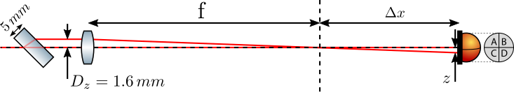
Figure 6: Added glass plate to induce an offset \(D_z\) of the incoming beam. It induces an offset \(z\) on the quadrant photodiode depending on how far it is from the focal plane \(\Delta x\)

Therefore, we should aim to position the quadrant photodiode in such a way that the change of read position on the quadrant photodiode is minimized when the glass window is added.

We want the quadrant photodiode to be positioned with an accuracy better than \(\Delta x = 0.4\,mm\), this corresponds to a change of position of the beam on the photodiode due to the glass windows of:

\begin{equation} D_y = \Delta x \cdot 1.6\,mm \approx 2.3\,\mu m \end{equation}

With a gain of the quadrant photodiode of about \(40\,\mu m/\text{unit}\) (see Section 3.3), we should aim to have a change of the readout on the quadrant photodiode due to the glass window less than:

\begin{equation} D_y < \frac{2.3\,\mu m}{40\,\mu m} \approx 0.06\,\text{unitless} \end{equation}

3. Photo-diodes Calibration

In order to compute the Y-Z position of the beam on the quadrant photodiodes from the voltages measured on the four quadrants, a calibration is required. The idea is to impose a know motion of the photodiode relative to the incoming beam. This is performed with an XYZ piezoelectric stage equipped with capacitive sensors.

The setup is described in Section 3.1. Then, the quadrant photodiode measuring the position of the beam is calibrated in Section 3.2 while the quadrant photodiode measuring the orientation of the beam is calibrated in Section 3.3.

3.1. Experimental Setup

The quadrant photodiode is fixed on an XYZ piezoelectric stage (see Figure 7). Using a DAC and a voltage amplifier, the quadrant photodiode can be displaced with respect to the incoming beam. The motion of the stage is measured with capacitive sensors.

By knowing both the motion of the quadrant photodiode with respect to the fixed beam, and the measured voltages on each quadrant, it is then possible to qualibrate the sensitivity of the quadrant photodiode.

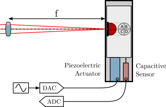
Figure 7: Calibration strategy for the quadrant photodiode - Schematic

Calibration of the capacitive sensors. The motion of the XYZ piezoelectric stage is measured with an external metrology (inductive probe with a resolution of \(0.5\,\mu m\)). The voltage on the piezo stage is adjusted in order to obtain a wanted motion as measured by the external metrology, and the voltage generated by the capacitive sensor is recorded.

The axes are:

x the horizontal axis perpendicular to the beam
y the vertical axis
z the beam axis

Table 8: Measured motion with external metrology and corresponding output voltages for the three axes
Motion [\(\mu m\)]	x [V]	y [V]	z [V]
-60	-4.77	-1.25	1.45
-30	-3.74	-0.29	2.46
0	-2.75	0.75	3.48
30	-1.74	1.78	4.49
60	-0.73	2.73	5.45

A linear fit is performed for each axis and the obtain capacitive sensor gains in \(\mu m/V\) are shown in Table 9.

Table 9: Estimated sensitivity of the capacitive sensor for the three axes
	x	y	z
Sensitivity [\(\u m/V\)]	29.8	29.9	29.9

The gain of the capacitive sensor output voltage is approximately \(30 \mu m/V\).

3.2. Position 4QD - Calibration

The quadrant photodiode used to measure the position of the beam is positioned in such a way that the incoming beam hits it at its center. Two scans with the PI stage are performed in the plane of the quadrant photodiode: one in the horizontal direction (corresponding to \(D_x\)) and in the vertical direction (corresponding to \(D_y\)).

These scans are sinusoidal displacements with an amplitude of around \(100\,\mu m\) with a frequency of 1 Hz. Four quantities are measured:

Px, Py: The \((x,y)\) position of the quadrant photodiode as measured by the capacitive sensors, in Volts
Dx, Dy: The \((x,y)\) position of the beam as measured by the quadrant photodiode, unitless

The beam position as measured by the quadrant photodiode during the two scans is shown in Figure 8.

%% Load Measurement Data
Dx = load('calib_4qd_Dx.mat'); % X scan
Dy = load('calib_4qd_Dy.mat'); % Y Scan

%% Capacitive Sensor Gain
G_capa = 30; % [um/V]

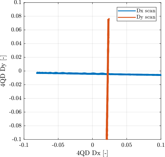
Figure 8: Position of the beam as measured by the quadrant photodiode during the two scans

Then, the relation between the measured stage displacement and the measured position on the beam is shown in Figure 9. Two things are be noted:

For the \(\pm 100\,\mu m\) scan, the relation is well linear
The gain for the two directions are slightly different. This could be an indication of a non circular beam

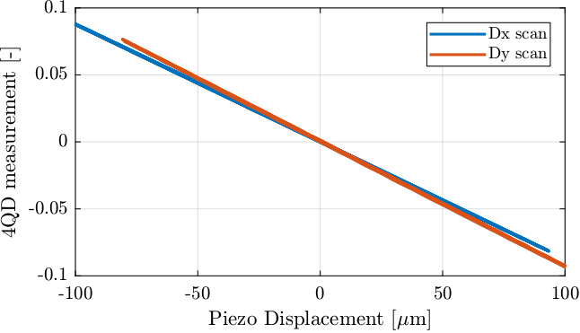
Figure 9: Quadrant Photodiode measurement as a function of its position

Then, a linear fit if performed. The result is shown in Figure 10.

%% Linear fit [um/-]
G_Dx = (Dx.Dx)\(G_capa*Dx.Px);
G_Dy = (Dy.Dy)\(G_capa*Dy.Py);

Figure 10: Linear and Sigmoid fit of the quadrant photodiode output to beam position

The gain of the photodiode in the linear region is:

Gain for Dx = -1141.8 [um/-]

Gain for Dy = -1071.8 [um/-]

The identified characteristics for the angular metrology are:

Gain of \(\approx 1100\,\mu\text{m}\)
Range of \(\approx 1100\,\mu\text{m}\)

3.3. Orientation 4QD - Calibration

The quadrant photodiode is first positioned at the focal plane of the lens. Two scans with the PI stage are performed in the plane of the quadrant photodiode: one in the horizontal direction (corresponding to \(R_x\)) and in the vertical direction (corresponding to \(R_y\)).

These scans are sinusoidal displacements with an amplitude of around \(100\,\mu m\) with a frequency of 1 Hz. Four quantities are measured:

Px, Py: The \((x,y)\) position of the quadrant photodiode as measured by the capacitive sensors, in Volts
Rx, Ry: The \((x,y)\) position of the beam as measured by the quadrant photodiode, unitless

%% Load Measurement Data
Rx = load('calib_4qd_Rx.mat');
Ry = load('calib_4qd_Ry.mat');

The beam position as measured by the quadrant photodiode during the two scans is shown in Figure 11.

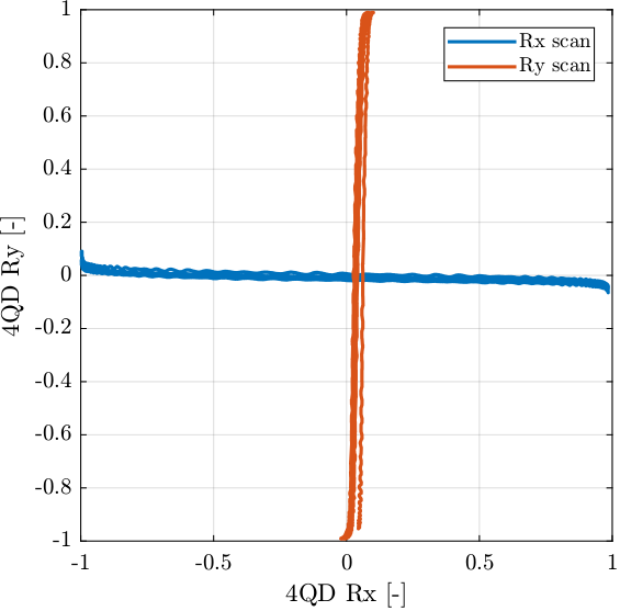
Figure 11: Position of the beam as measured by the quadrant photodiode during the two scans

The relation between the piezoelectric stage motion and the quadrant photodiode measured position is shown in Figure 12.

Several things can be noted from Figure 12:

The full stroke of the quadrant photodiode has been scanned
The approximate beam diameter is about \(100\,\mu m\)
The linear region is around \(\pm 20\,\mu m\)

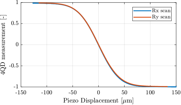
Figure 12: Quadrant Photodiode measurement as a function of its position

Then, a linear fit if performed near the origin.

%% Estimation of linear region
i_Rx = Rx.Rx < 0.1 & Rx.Rx > -0.1;
i_Ry = Ry.Ry < 0.1 & Ry.Ry > -0.1;

%% Linear fit near origin
G_Rx = (Rx.Rx(i_Rx))\(G_capa*Rx.Px(i_Rx)); % Gain in [um/-]
G_Ry = (Ry.Ry(i_Ry))\(G_capa*Ry.Py(i_Ry)); % Gain in [um/-]

This corresponds to the gain of the photodiode in the linear region:

Gain for Rx = -39.8 [um/-]

Gain for Ry = -40.4 [um/-]

A sigmoid fit is also performed that better represents the behavior of the quadrant photodiode.

%% Sigmoid Fit
A1 = -1;
A2 =  1;
k = -19.5;
xa = 0;

x = -150:1:150; % Linear position [um]
y = (A1-A2)./(1 + exp((x-xa)/k)) + A2; % Sigmoid Function [-]

The two fits are compared in Figure 13.

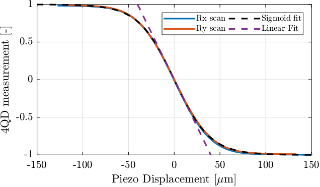
Figure 13: Linear and Sigmoid fit of the quadrant photodiode output to beam position

The beam radius can be estimated from the above plot.

%% Beam Radius (1/e2) estimation
[~, i_Rx_high] = min(abs(Rx.Rx - 0.95));
[~, i_Rx_low]  = min(abs(Rx.Rx + 0.95));
Rx_radius = 30*(Rx.Px(i_Rx_low) - Rx.Px(i_Rx_high))/2;

[~, i_Ry_high] = min(abs(Ry.Ry - 0.95));
[~, i_Ry_low]  = min(abs(Ry.Ry + 0.95));
Ry_radius = 30*(Ry.Py(i_Ry_low) - Ry.Py(i_Ry_high))/2;

Beam Radius (1/e2) = 67 [um]

The expected beam radius (\(1/e^2\)) from optical simulation is \(54\,\mu m\) so we are pretty close.

Now, let’s translate the measurement into angle of the incoming beam.

The relation between the position of the beam on the quadrant photodiode \((x, y)\) and the angle of the incoming beam \((Rx, Ry)\) is:

\begin{align} Rx &= \frac{x}{f} \\ Ry &= \frac{y}{f} \end{align}

with \(f = 400\,mm\) the focal of the lens.

f = 0.4; % Focal of lens [m]

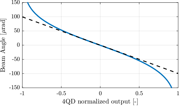
Figure 14: Incoming beam angle as a function of the quadrant photodiode normalized output

The obtained gain of the quadrant photodiode for the angular measurement is:

Gain for Rx = -99.5 [urad/-]

Gain for Ry = -101.0 [urad/-]

The identified characteristics for the angular metrology are:

Gain of \(\approx 100\,\mu\text{rad}\)
Linear range of \(\approx 100\,\mu\text{rad}\)

4. Noise Measurement

In this section, it is wished to characterize the high frequency behaviour of the metrology setup (i.e. above 1 Hertz). The low frequency behavior (i.e. drifts) will be studied in Section 6.

To do so, the noise of several components are measured:

The Analog to Digital converters (Section 4.1)
The effect on long coaxial cables (Section 4.2)
The transimpedance amplifier (Section 4.3)
The effect of the super luminescent diode (Section 4.4)
The mechanical noise (Section 4.5)

The noise budgeting is finally performed in Section 5. Conclusions on the current limitations of the laser setup can be drawn, and improvements are proposed in Section 5.1.

4.1. ADC Noise

The IO131 Speedgoat board is containing 16 ADC with an input range of \(\pm 5\,V\) with \(16\) bits of resolution (doc).

One LSB (“Least Significant Bit”) then corresponds to:

ADC LSB = 2.54 [nrad] / 25.43 [nm]

The quantization noise spectral spectral density is flat (i.e. can be approximated as white noise) and can be estimated as follows:

\begin{equation} \Gamma_{\text{ADC}} (\omega) = \sqrt{\frac{q^2}{12 f_s}} \text{ in } \left[ \frac{V}{\sqrt{Hz}} \right] \end{equation}

with:

\(q = \frac{\Delta V}{2^n} = 0.15\,mV\) the resolution of the ADC
\(\Delta V = 10\,V\) is the full range of the ADC
\(n = 16\) is the number of ADC’s bits
\(f_s = 10\,kHz\) is the sample frequency

ASD of quantization noise is 0.44 uV/sqrt(Hz) which corresponds to 0.01 nrad/sqrt(Hz) / 0.07 nm/sqrt(Hz)

Over a bandwidth of 5 kHz, this corresponds to a noise of:

Quantization noise = 0.52 [nrad RMS] / 5.19 [nm RMS]

Quantization noise should not be an issue here. However, there are several ways to improve the quantization noise:

Increasing the sampling frequency (20kHz can be achieved with the Speedgoat)
Using ADC oversampling (x4 up to x64). An oversampling of x16 is currently used.
Using an ADC with better characteristics

On top of the quantization noise, the ADC may have some input voltage noise that is higher than the quantization noise. This can be estimated using the following setup:

Experimental Setup:

\(50\,\Omega\) terminator are directly connected to the ADC inputs
the ADC output (i.e. digital) is recorded and the amplitude spectral density is computed

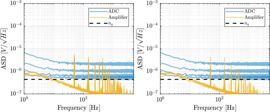
The power spectral density of the measured voltage is computed. The amplitude spectral density (ASD) of the ADC are shown in Figure 15.

The measured ADC noise varies a little bit from one unit to the other, but it could be a signal processing artifact. We are probably limited by the quantization noise here.

%% Compute PSD of measured voltage
adc.win = hanning(ceil(2*adc.Fs)); % Hannning Windows

[adc.Pur, adc.f] = pwelch(detrend(adc.Dur, 0), adc.win, [], [], 1/adc.Ts);
[adc.Pul, ~]     = pwelch(detrend(adc.Dul, 0), adc.win, [], [], 1/adc.Ts);
[adc.Pdr, ~]     = pwelch(detrend(adc.Ddr, 0), adc.win, [], [], 1/adc.Ts);
[adc.Pdl, ~]     = pwelch(detrend(adc.Ddl, 0), adc.win, [], [], 1/adc.Ts);

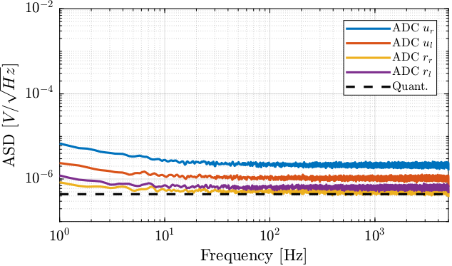
Figure 15: Amplitude Spectral Density of ADC noise

Then, we can estimate the effect of the ADC noise on the angle/position of the beam as measured by the quadrant photodiode.

%% Estimated signal on the normalized quandrant photodiode output
adc.x = (adc.Dur + adc.Ddr - adc.Dul - adc.Ddl)./(adc.Dur + adc.Ddr + adc.Dul + adc.Ddl + 4*Vm);

%% Power Spectral Density of the measured signal in [nm^2/Hz and nrad^2/Hz]
[adc.P_Dx, ~] = pwelch(detrend(1e9*Gd*adc.x, 0), adc.win, [], [], 1/adc.Ts);
[adc.P_Rx, ~] = pwelch(detrend(1e9*Gr*adc.x, 0), adc.win, [], [], 1/adc.Ts);

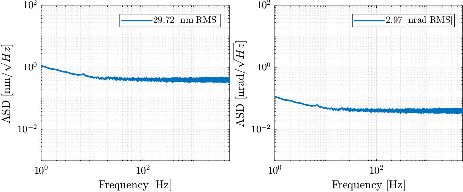
Figure 16: Induced ASD of angle and position of the beam

4.2. Noise Coming from long coaxial cables

Long (5m) coaxial cables are used between the transimpedance amplifiers and the ADC. Such cable could be an additional source of noise due to electromagnetic interference.

This additional noise is estimated using the following experimental setup.

Experimental Setup:

\(50\,\Omega\) terminator are connected to the ADC inputs through the 5m long BNC cable
the ADC output (i.e. digital) is recorded and the amplitude spectral density is computed

The measured voltage by the ADC are loaded.

%% Measurement with 50 Ohm terminators after 5m cable
cable = load('meas_noise_cable.mat');

And their power spectral density computed.

%% Compute PSD of measured voltage
cable.win = hanning(ceil(2*cable.Fs)); % Hannning Windows

[cable.Pur, cable.f] = pwelch(detrend(cable.Dur, 0), cable.win, [], [], 1/cable.Ts);
[cable.Pul, ~]       = pwelch(detrend(cable.Dul, 0), cable.win, [], [], 1/cable.Ts);
[cable.Pdr, ~]       = pwelch(detrend(cable.Ddr, 0), cable.win, [], [], 1/cable.Ts);
[cable.Pdl, ~]       = pwelch(detrend(cable.Ddl, 0), cable.win, [], [], 1/cable.Ts);

The ASD of the ADC with and without the 5m cable are compared in Figure 17.

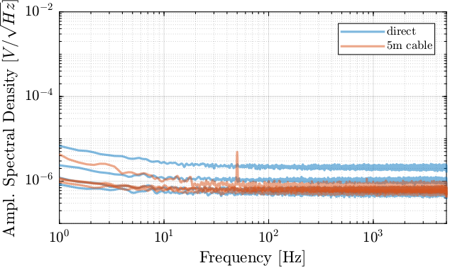
Figure 17: Comparison of the Amplitude Spectral Density of the ADC with and without the 5m cable

Except from a small 50Hz pickup by the 5m cable, having 5m cables does not seems to add any significant noise to the signal.

4.3. Transimpedance Amplifier Noise

In order to measure the noise of the transimpedance amplifier, the following experimental setup is used:

Experimental Setup:

the transimpedance amplifier input is connected to the quadrant photodiode which is not receiving any light
the transimpedance amplifier output is connected to a low noise voltage amplifier (Femto) with a gain of 1000
the output of the voltage amplifier is connected to the ADC
the ADC output (i.e. digital) is recorded and the amplitude spectral density is computed

We can first estimate the noise of the transimpedance amplifier with a simple calculation:

The gain of the transimpedance amplifier is \(100\,kV/A\). Therefore, the feedback resistance in the amplifier (equal to \(R_f = 100\,k\Omega\)) creates a Johnson noise (white noise) that corresponds to a current noise of:

\begin{equation} \Gamma_i = \sqrt{\frac{4 k T}{R_f}} \approx 0.4\, pA/\sqrt{Hz} \end{equation}

Which is close to the specified input current noise \(\Gamma_i = 0.36\,pA/\sqrt{\text{Hz}}\) found in the documentation.

In terms of output voltage noise:

\begin{equation} \Gamma_v = 100\cdot10^3 \cdot \Gamma_i \approx 40 nV/\sqrt{Hz} \end{equation}

This is smaller than the quantization noise of the ADC, so it should not be a limitation. Let’s verify that.

The measured voltages are loaded.

%% Load measured voltages on the 4 quadrants
ampl = load('meas_noise_transimpedance_amplifier.mat')

And the measured voltages are divided by 1000 to take into account the gain of the voltage amplifier.

Then, the power spectral density of the measured voltages are computed, and shown in Figure 19. It is clear that the transimpedance amplifier noise is bellow the noise of the ADC and therefore is not an issue. There is however some 50Hz (and odd harmonics), care should be taken to minimize this pickup of main’s noise.

%% PSD of measured voltage is computed
ampl.win = hanning(ceil(2*ampl.Fs)); % Hannning Windows

[ampl.Pdur, ampl.f] = pwelch(detrend(ampl.Dur, 0), ampl.win, [], [], 1/ampl.Ts);
[ampl.Pdul, ~]      = pwelch(detrend(ampl.Dul, 0), ampl.win, [], [], 1/ampl.Ts);
[ampl.Pddr, ~]      = pwelch(detrend(ampl.Ddr, 0), ampl.win, [], [], 1/ampl.Ts);
[ampl.Pddl, ~]      = pwelch(detrend(ampl.Ddl, 0), ampl.win, [], [], 1/ampl.Ts);
[ampl.Prur, ~]      = pwelch(detrend(ampl.Rur, 0), ampl.win, [], [], 1/ampl.Ts);
[ampl.Prul, ~]      = pwelch(detrend(ampl.Rul, 0), ampl.win, [], [], 1/ampl.Ts);
[ampl.Prdr, ~]      = pwelch(detrend(ampl.Rdr, 0), ampl.win, [], [], 1/ampl.Ts);
[ampl.Prdl, ~]      = pwelch(detrend(ampl.Rdl, 0), ampl.win, [], [], 1/ampl.Ts);

The corresponding noise on the measured displacement and orientation of the beam are computed.

%% Estimated signal on the normalized quandrant photodiode output
ampl.Dx = (ampl.Dur + ampl.Ddr - ampl.Dul - ampl.Ddl)./(ampl.Dur + ampl.Ddr + ampl.Dul + ampl.Ddl + 4*Vm);
ampl.Rx = (ampl.Rur + ampl.Rdr - ampl.Rul - ampl.Rdl)./(ampl.Rur + ampl.Rdr + ampl.Rul + ampl.Rdl + 4*Vm);

%% Induced Power Spectral Density in [nm^2/Hz and nrad^2/Hz]
[ampl.P_Dx, ~] = pwelch(detrend(1e9*Gd*ampl.Dx, 0), ampl.win, [], [], 1/ampl.Ts);
[ampl.P_Rx, ~] = pwelch(detrend(1e9*Gr*ampl.Rx, 0), ampl.win, [], [], 1/ampl.Ts);

4.4. Laser Source Noise

In order to see if the light source (super-luminescent diode) itself is inducing some measurement noise, the following measurement setup is performed.

Experimental Setup:

the quadrant photodiode and the laser head are rigidly fixed to the same frame such that there is no relative motion between the two
the laser beam is pointed at the 4QD center

This has been done both for the position quadrant photodiode as well as for the orientation quadrant photodiode.

%% Load measured voltages on the 4 quadrants
laser = load('meas_noise_laser.mat'); % Dx, Dy, Rx and Ry are unitless

The power spectral density of the measured signals are computed.

%% PSD of measured voltage is computed
laser.win = hanning(ceil(2*laser.Fs)); % Hannning Windows

[laser.P_Dx, laser.f] = pwelch(detrend(1e9*Gd*laser.Dx, 0), laser.win, [], [], 1/laser.Ts);
[laser.P_Dy, ~]       = pwelch(detrend(1e9*Gd*laser.Dy, 0), laser.win, [], [], 1/laser.Ts);
[laser.P_Rx, ~]       = pwelch(detrend(1e9*Gr*laser.Rx, 0), laser.win, [], [], 1/laser.Ts);
[laser.P_Ry, ~]       = pwelch(detrend(1e9*Gr*laser.Ry, 0), laser.win, [], [], 1/laser.Ts);

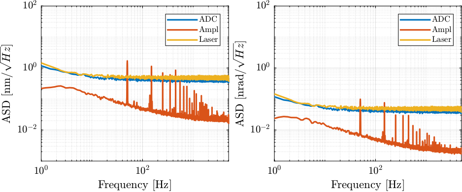
Figure 18: Amplitude Spectral density of the measured position and orientation due to the laser noise

The noise coming from the light source is probably small compared with the ADC noise. To be sure about that, another measurement with an higher quality ADC could be done.

The effect of the laser noise on the measured position and orientation are computed.

%% Estimated signal on the normalized quandrant photodiode output
laser.x = (laser.ur + laser.dr - laser.ul - laser.dl)/(laser.ur + laser.dr + laser.ul + laser.dl + 4*Vm);

%% Power Spectral Density
[laser.P_Dx, ~] = pwelch(detrend(Gd*laser.x, 0), laser.win, [], [], 1/laser.Ts);
[laser.P_Rx, ~] = pwelch(detrend(Gr*laser.x, 0), laser.win, [], [], 1/laser.Ts);

4.5. Mechanical Noise

If there is some relative motion between the plate holding the light source and the plate holding the quadrant photodiodes, it will be seen in the measured motion. This can be seen as “mechanical noise”.

In order to estimate this “mechanical noise”, the following setup is performed.

Experimental Setup:

Everything is setup as for the final measurement except that the DCM is not present:
- The two four quadrant diodes are aligned on fixed one one optical table
- The Laser is fixed to another optical table

The measurement data are loaded, and the time domain data are shown in Figure 19. Several things can be observed:

there are some low frequency drifts (that will be studied in Section 6)
there are some high frequency motion, probably due to resonances of the metrology supports
There is less motion on \(R_x\) than on \(R_y\)

%% Load Measurement Data
mech = load('meas_noise_metrology_high_freq.mat');

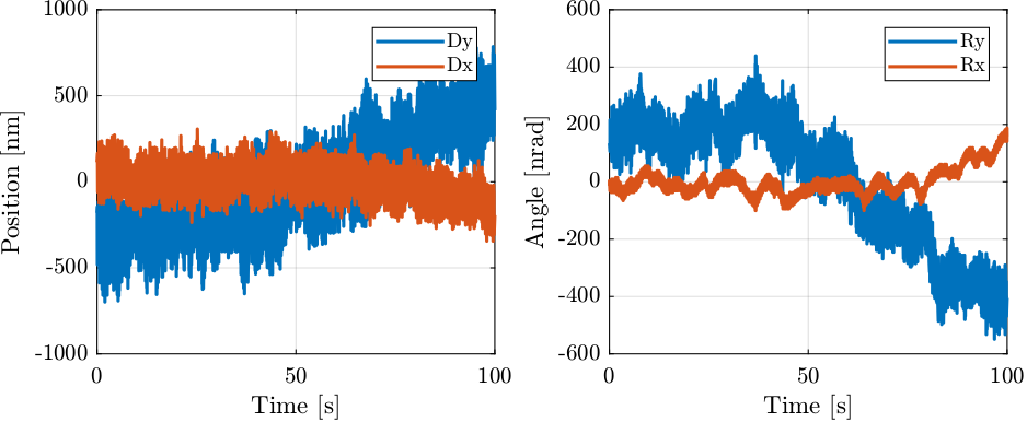
Figure 19: Measured pose of the beam as a function of time

The power spectral density of the measured motion is computed. The contribution of the mechanical noise is compared with the other contribution in Figure 20 for the translations and in Figure 21 for the rotations.

%% Power Spectral Density
mech.win = hanning(ceil(2*mech.Fs)); % Hannning Windows

[mech.P_Dx, mech.f] = pwelch(detrend(1e9*Gd*mech.Dx, 0), mech.win, [], [], 1/mech.Ts);
[mech.P_Dy, ~]      = pwelch(detrend(1e9*Gd*mech.Dy, 0), mech.win, [], [], 1/mech.Ts);
[mech.P_Rx, ~]      = pwelch(detrend(1e9*Gr*mech.Rx, 0), mech.win, [], [], 1/mech.Ts);
[mech.P_Ry, ~]      = pwelch(detrend(1e9*Gr*mech.Ry, 0), mech.win, [], [], 1/mech.Ts);

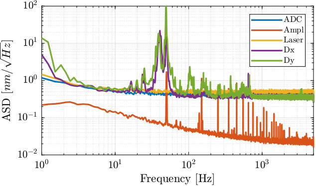
Figure 20: Amplitude Spectral Density of the measured position of the beam

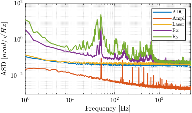
Figure 21: Amplitude Spectral Density of the measured rotation of the beam

From Figure 20 and 21, it is clear that the mechanical noise is the main source of noise up to 1kHz.

5. Noise budgeting

Several sources of noise have been identified:

ADC noise (quantization and voltage input noise)
Transimpedance amplifier noise
Light source noise
Mechanical noise

The effect of these sources of noise on the quadrant photodiode measurement are now compared in Figure 22 for translations and in Figure 23 for rotations.

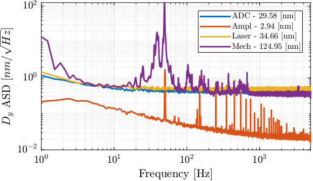
Figure 22: Noise Budgeting for the measured translations (RMS values integrated from 1Hz to 5kHz are noted in the legend)

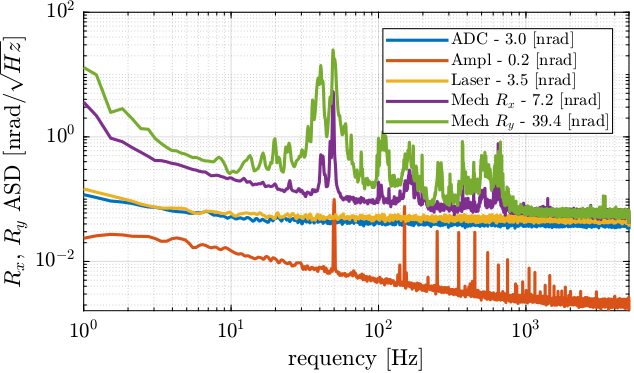
Figure 23: Noise Budgeting for the measured rotations (RMS values integrated from 1Hz to 5kHz are noted in the legend)

Regarding translations (see Figure 22), the main limitation from 20Hz to 800Hz is the relative motion between the two optical plates. Above 800Hz, the noise is dominated by the ADC. Between a few Hertz and 20Hz, it seems that the limitation comes from the ADC. Below that, mechanical drifts are probably the limitation.

Regarding rotations (see Figure 23), from DC up to 800Hz, the clear limitation is coming from the relative motion between the two optical plates. Above 800Hz, the noise is dominated by the ADC, but remains very small. It should be noted that there is much more “mechanical noise” on \(R_y\) than on \(R_x\)

The measured RMS values (integrated from 1Hz up to 5kHz) are summarized in Table 10.

Table 10: RMS value of measured beam position/orientation due to several factors
	ADC	Amplifier	Laser	Mechanical
Dy [nm RMS]	29.6	2.9	34.7	124.9
Rx [nrad RMS]	3.0	0.2	3.5	7.2
Ry [nrad RMS]	3.0	0.2	3.5	39.4

5.1. Possible Improvements

5.1.1. Damping of natural frequency

If the mode shapes for the two problematic modes are well identified, it would be possible to damp them effectively. This can be done for instance using Tuned Mass Dampers.

5.1.2. Low pass filtering

In order to see how filtering of high frequency noise (similar to averaging) can lower the noise in the measurement, the Cumulative Amplitude Spectrum (CAS) of the measured signals is computed.

It is shown in Figure 24, and we can see that the resonances at 40 Hz and 50 Hz are a major contribution of the total RMS value. Therefore, if the signal can be low pass filtered with a cut-off frequency before 40Hz, the RMS value of the obtained signal can be well lowered. The price to pay is that the useful part of the signal above 40Hz will also be filtered out. Therefore, this can only be done if a measurement bandwidth below 40Hz is acceptable.

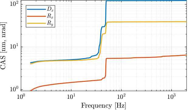
Figure 24: Cumulative Amplitude Spectrum (CAS) of the measured position/orientation

5.1.3. Measurement and compensation of high frequency vibrations

The high frequency “mechanical noise” (i.e. vibrations) could be measured with an external metrology and compensated in real time.

This could be done using interferometers, or using another similar metrology currently used (laser, lens and quadrant photodiode).

6. Stability Measurement

If there is a relative motion between the laser and the quadrant diode (i.e. between the two optical plates), depending on the considered motion it could will be translated into variation of signals on the quadrant diodes and therefore could induce errors on the measurement.

There are 6 possible relative motion between the two plates, and their effects on the measurement are summarized in Table 11.

Table 11: Possible relative motion between optical tables and their effect on the measurement
Motion	Laser Plate	Photodiode Plate
\(D_x\)	Not an issue	Not an issue
\(D_y\)	Not an issue	Not an issue
\(D_z\)	Directly translated as Dz measurement	Directly translated as -Dz measurement
\(R_x\)	Not an issue if around laser axis. Otherwise, translate as Dz measurement	Not an issue if around laser axis. Otherwise, translate as Dz measurement
\(R_y\)	Translate to Ry measurement and Dz with lever arm between rotation axis and the second crystal	Translate to Ry
\(R_z\)	Translate to Rx measurement	Translate to Rx measurement

For the most stringent requirements (measurement of dRx and dRy motion of the crystal), the \(R_y\) and \(R_z\) relative motion of the two optical plates should be controlled to better than what we want to measure. This means that the relative motion between the two plates should be controlled to better than what is listed in Table 12.

Table 12: Requirement on the relative motion between the two optical plates
Motion	Stability (5 min)	Vibrations (200Hz BW)
\(R_y\)	100 nrad	20 nrad RMS
\(R_z\)	200 nrad	40 nrad RMS

6.1. First Measurement of stability

The setup is schematically represented in Figure 25. As it is expected that thermal drift will be the main issue, one temperature sensor is fixed on each pillar (8 in total).

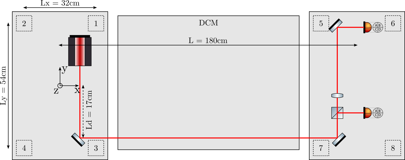
Figure 25: Schematic of the measurement setup. The number are representing the temperature sensors on each pillar

6.1.1. Measured Beam motion

The motion of the beam is measured by the two quadrant photodiodes during 5 hours with a sampling time of 10 seconds. The 8 temperature sensors are recorded at the same time.

The measured rotation/translation of the beam by the two quadrant photodiode are shown in Figures 26 and 27.

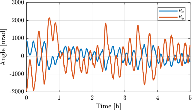
Figure 26: Measured rotational drifts of the beam as measured by the quadrant photodiode

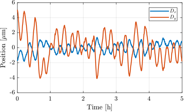
Figure 27: Measured translational drifts of the beam as measured by the quadrant photodiode

From Figures 26 and 27, it is clear that the motion mainly contains one period that is estimated to be around 13 minutes.

The angular drift rate (number of nano-radians per minute) can be estimated from the measurement. The results are shown in Figure 28. It is shown that the drifts can be as high as 500 nrad/min for \(R_y\) and 250 nrad/min for \(R_x\) which is much more than the specifications.

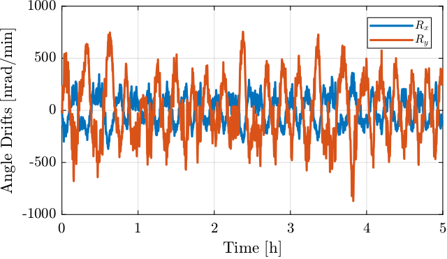
Figure 28: Measured Angular drift rate

The results are summarized in Table 13.

Table 13: Estimated drifts amplitude and worst drift over one minute
	Dy [\(\mu m\)]	Rx [nrad]	Ry [nrad]
Amplitude	2.7	480.8	1187.4
Worst Drift [\(\text{min}^{-1}\)	1.3	232.4	573.9

From Figures 26 and 28 and Table 13, it is clear that the drifts are way too high compared to the specifications.

It can be seen that the positions drifts in figure 27 are very similar to the rotational drifts on Figure 26. This can be explained by the large rotational motion and the quite large lever arm between the two pillars.

Indeed, if the measured rotational motion is multiplied by the lever arm, we find that it matches very well the measured translation of the beam (Figure 29).

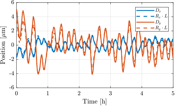
Figure 29: Comparison of measured \(D_x\) and \(D_y\) with the effect of Rx and Ry due to the lever arm between the laser and the photodiodes

6.1.2. Measured Temperature

The 8 temperatures sensors (one fixed on each pillar, as shown in Figure 25) are also recorded.

The measured temperatures of each pillar are shown in Figure 30.

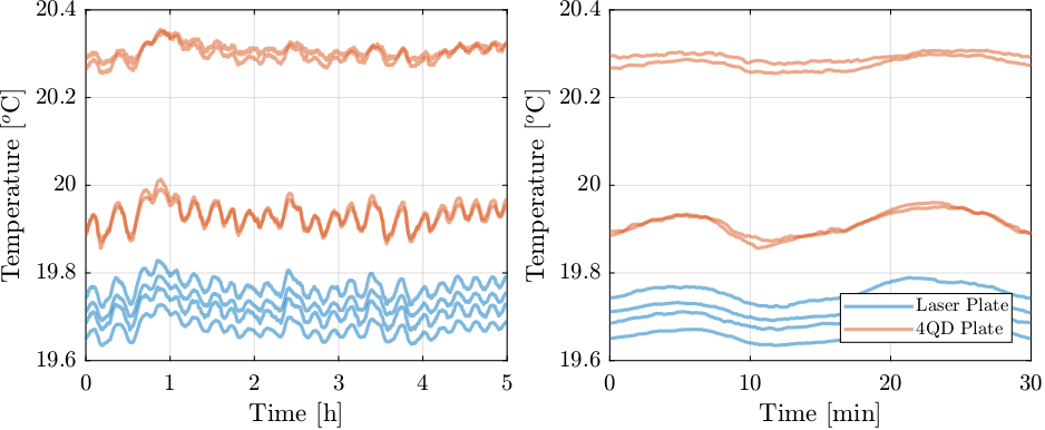
Figure 30: Mean temperature fluctuation of pillars

From Figure 30, we can see that the temperature of pillars supporting the quadrant photodiodes are higher than the temperature of the pillars supporting the laser. Especially two of the four pillars which are the number 6 and 8. This can be explained by the fact that these two pillars are closed to the “blue rack” containing a lot of heating elements.

It can also be seen that the temperature is fluctuating with a period of 13 minutes, similarly to the measured motion of the beam by the quadrant photodiodes. This is an strong indication that the measured motion is due to thermal effects.

6.1.3. Thermal Model

Now that we now that the measured motion of the beam is due to thermal effects, we can try to correlate the temperature measurements with the motion of the beam. To do that, a thermal model of the metrology supports has to be developed.

From the geometry in Figure 25, we can estimate the motion of the pillars as follow (\(l\) stands for “laser” and \(p\) for “photodiode”):

\begin{align} d_{z,l} &= \alpha H \left( \frac{T_1 + T_2 + T_3 + T_4}{4} \right) \\ \theta_{x,l} &= \frac{\alpha H}{L_y} \left( \frac{T_1 + T_2}{2} - \frac{T_3 + T_4}{2} \right) \\ \theta_{y,l} &= \frac{\alpha H}{L_x} \left( \frac{T_1 + T_3}{2} - \frac{T_2 + T_4}{2} \right) \\ d_{z,p} &= \alpha H \left( \frac{T_1 + T_2 + T_3 + T_4}{4} \right) \\ \theta_{x,p} &= \frac{\alpha H}{L_y} \left( \frac{T_5 + T_6}{2} - \frac{T_7 + T_8}{2} \right) \\ \theta_{y,p} &= \frac{\alpha H}{L_x} \left( \frac{T_6 + T_8}{2} - \frac{T_5 + T_7}{2} \right) \end{align}

with:

\(\alpha\) the coefficient of linear thermal expansion in \(m/m/^oC\) (equal to \(\approx 12\, \mu m/m/^oC\) for steel)
\(H\) the height of the pillars \(\approx 1.2\,m\)
\(L_x\) and \(L_y\) the distance between the pillars as shown in Figure 25
\(T_i\) the temperature of the i’th pillar

The effect of the metrology plate motion induced by thermal drifts on the measured beam motion can be estimated using the following formulas:

\begin{align} R_y &= \theta_{y,l} - \theta_{y,p} \\ D_z &= d_{z,l} - d_{z,p} + L \theta_{y,l} + L_d (\theta_{y,l} - \theta_{x,l}) \end{align}

with \(L\) the distance between the two metrology plates.

Note that \(R_x\) cannot be estimated from the temperature sensors.

6.1.4. Comparison of the measured temperature and beam motion

The geometry of the setup is defined below (see Figure 25 for naming conventions).

%% Pilar Geometry
H = 1.2; % Pillar Height [m]
Lx = 0.32; % [m]
Ly = 0.54; % [m]
Ld = 0.17; % [m]
L = 1.8; % [m]

alpha = 12e-6; % Coefficient of Linear Thermal Expansion [um/m/oC]

The estimated beam motion due to temperature drifts are computed from equations derived in Section 6.1.3.

%% Estimation of motion due to temperature drifts
Ry_temp = alpha*H/Lx*(((temp(:,1)+temp(:,3))/2 - (temp(:,2)+temp(:,4))/2) - ... % Rotation on 1st pillar
                      ((temp(:,6)+temp(:,8))/2 - (temp(:,5)+temp(:,7))/2)); % Rotation of 2nd pillar

Dz_temp = alpha*H*(((temp(:,1) + temp(:,2) + temp(:,3) + temp(:,4))/4) - ... % Pure Translation
                   ((temp(:,5) + temp(:,6) + temp(:,7) + temp(:,8))/4)) + ...
          L*alpha*H/Lx*((temp(:,1)+temp(:,3))/2 - (temp(:,2)+temp(:,4))/2) + ... % Due to Laser Ry motion
         -Ld*alpha*H/Ly*(((temp(:,1)+temp(:,2))/2 - (temp(:,3)+temp(:,4))/2) - ...
                         ((temp(:,5)+temp(:,6))/2 - (temp(:,7)+temp(:,8))/2)); % Due to Rx of both platforms

The estimation for \(R_y\) is compared with the measurement in Figure 31.

From Figure 31, it can be seen that there is a relatively good agreement between the measurement and the estimation from the temperature. This confirms that the measured \(R_y\) tilt of the beam by the photodiodes is due to tilts of the optical plates due to thermal motion of the pillars.

More precisely, this is due to difference of thermal expansion of the two sets of pillars responsible of the \(R_y\) motion.

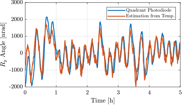
Figure 31: Comparison of measured Ry motion of the beam and the estimated one from temperature

From Figure 32, it seems that there is a small delay between the measured temperature and the quadrant photodiode readout. This is logical as thermal drifts are not instant.

This drifts can be estimated from the data:

Time delay = 60 [s]

The drifts estimation from the temperature is now delayed by one minute and compared with the quadrant photodiode readout in Figure 32. The remaining motion (measured minus delayed estimate) is also shown in Figure 32.

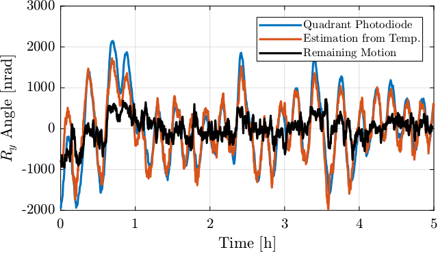
Figure 32: Comparison of measured \(R_y\) motion of the beam and the estimated one from temperature delayed by one minute

From Figure 32, it can be seen that there is a relatively good agreement between the \(R_y\) drifts estimated by the temperature sensors and the measured \(R_y\) by the quadrant photodiodes. When subtracting the two, is lowers the amplitudes but adds some fastest variations that are probably due to the temperature noise sensor.

Let’s now see if the \(R_y\) drifts are due to drifts of the Laser plate or due to drifts of the quadrant photodiode plate.

This is shown in Figure 33, and it can be seen that much of the drifts are due to the pillars holding the optical plate where the quadrant photodiodes are fixed.

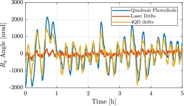
Figure 33: \(R_y\) drifts to the drifts of the two optical plates

The \(D_y\) measured motion of the beam is compared with the estimation from temperature of each pillar in Figure 34.

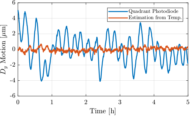
Figure 34: Comparison of measured \(D_y\) motion of the beam and the estimated one from temperature

As shown in Figure 35, the estimation from the temperature sensors of the \(D_y\) motion of the beam is not correct. It is probably be due to a too simplistic thermal model.

6.1.5. Optimization of temperature compensation

As was shown in Figure 32, the temperature sensors are quite noisy. Therefore, if the drifts are compensated using the temperature sensors, this could lead to an add of noisy estimated motion of the beam.

In order to avoid this, the temperature can be low pass filtered. A FIR filter can be used, with an added delay equal to the delay between the read temperature and the effect on the quadrant photodiode. Therefore, the filtered estimation from the temperature and the quadrant photodiode readout should be in phase.

The FIR filter order is chosen to be 12 such that it will induce a delay corresponding to 6 time steps (i.e. 60 seconds). It is designed as follows:

%% FIR with Linear Phase
Fs = 0.1; % Sampling Frequency [Hz]
B_fir = firls(12, ... % Filter's order
              [0 1/60/10/(Fs/2) 1/60/2/(Fs/2) 1], ... % Frequencies [Hz]
              [1 1          0          0]); % Wanted Magnitudes

The comparison between the raw signal and the filtered one is done in Figure 35.

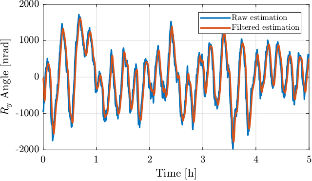
Figure 35: Comparison of the raw estimated \(R_y\) and the filtered one

Now the \(R_y\) motion measured by the quadrant photodiodes as well as the filtered estimation from the temperature sensors are compared in Figure 36. A slight improvement can be observed as compared with the un-filtered estimation (see Figure 32).

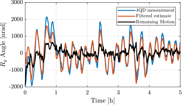
Figure 36: Comparison of the photodiode \(R_y\) measurement and the filtered estimate from temperature. The remaining motion is also shown

6.2. Measurement with isolated pillars

In order to limit the thermal drifts of the pillars a measurement has been performed with some “thermal protection” around the pillars. First, a aluminum foil is fixed around the pillars to help homogenize the temperature of each pillar. Then, bubble wrap is used to limit the thermal transfer between the air of the lab to the pillars.

6.2.1. Measurement with isolated pillars

The temperature of the 8 pillars are compared in Figure 37. The temperature of each set of four “isolated” pillars are closer from each other than before (see Figure 30). However, the relative temperature between two pillars supporting the same optical plate may not have improved.

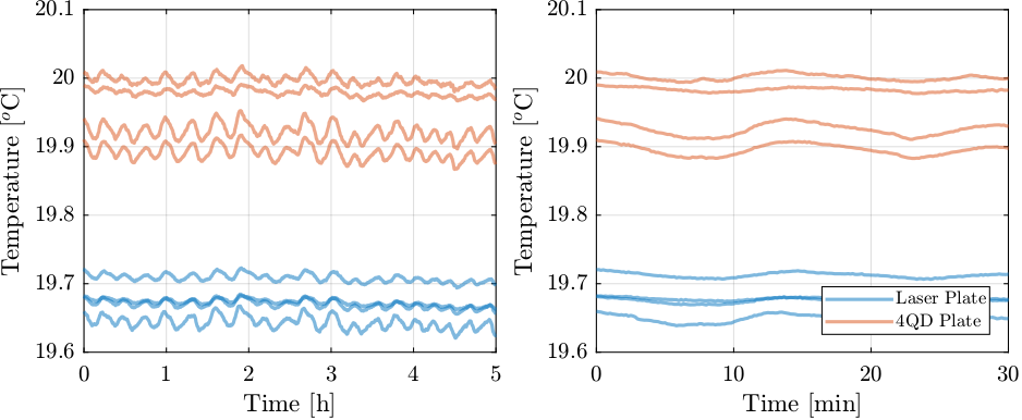
Figure 37: Mean temperature fluctuation of pillars

%% Pilar Geometry
H = 1.2; % Pillar Height [m]
Lx = 0.32; % [m]
Ly = 0.54; % [m]
Ld = 0.17; % [m]
L = 1.8; % [m]

alpha = 12e-6; % Coefficient of Linear Thermal Expansion [um/m/oC]

%% Estimation of motion due to temperature drifts
Ry_temp = alpha*H/Lx*(((temp(:,1)+temp(:,3))/2 - (temp(:,2)+temp(:,4))/2) - ... % Rotation on 1st pillar
                      ((temp(:,6)+temp(:,8))/2 - (temp(:,5)+temp(:,7))/2)); % Rotation of 2nd pillar

Dz_temp = alpha*H*(((temp(:,1) + temp(:,2) + temp(:,3) + temp(:,4))/4) - ... % Pure Translation
                   ((temp(:,5) + temp(:,6) + temp(:,7) + temp(:,8))/4)) + ...
          L*alpha*H/Lx*((temp(:,1)+temp(:,3))/2 - (temp(:,2)+temp(:,4))/2) + ... % Due to Laser Ry motion
         -Ld*alpha*H/Ly*(((temp(:,1)+temp(:,2))/2 - (temp(:,3)+temp(:,4))/2) - ...
                         ((temp(:,5)+temp(:,6))/2 - (temp(:,7)+temp(:,8))/2)); % Due to Rx of both platforms

The measured rotation/translation of the beam by the two quadrant photodiode are shown in Figures 26 and 27.

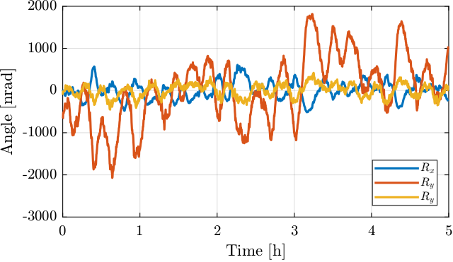
Figure 38: Measured rotational drifts of the beam as measured by the quadrant photodiode

6.2.2. Evaluation of the benefits of adding thermal insulation

The measured temperature with and without thermal protection are now compared.

The mean temperature of the four pillars supporting the laser plate and the photodiode plate are compared in Figure 39. It is clear that the thermal protection helps decreasing the fluctuation of the mean temperature of the four pillars.

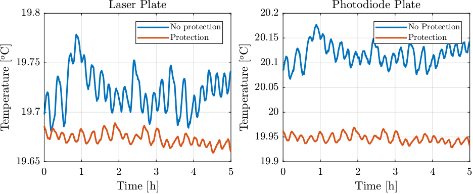
Figure 39: Temperature mean of the pillars supporting the two plates - comparison with and without thermal protection

Now, let’s see if it also helps reducing the temperature gradient between pillars supporting the same optical plate. Indeed, this is more important than the mean fluctuation of the four pillars are this is what is inducing tilts of the optical plate. The results are shown in Figure 40, and there is not a clear indication of improvement.

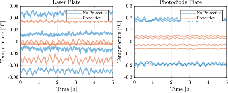
Figure 40: Temperature difference of the pillars supporting the two plates - comparison with and without thermal protection

This is confirmed by looking at the RMS values of the pillar temperature variations with respect to the mean temperature of the pillars supporting the same optical plate in Table 14.

Table 14: Root Mean Square value of the fluctuation of each pillar temperature with respect to the mean of the four pillars supporting the same optical plate. The results are in mK RMS
	No Protection	Protection
1 (Laser)	1.8	2.5
2 (Laser)	2.7	3.6
3 (Laser)	2.6	1.2
4 (Laser)	2.3	0.5
5 (Photodiodes)	10.4	2.4
6 (Photodiodes)	5.8	4.4
7 (Photodiodes)	5.2	3.8
8 (Photodiodes)	10.1	2.4

Finally, if we compare with measured tilt by the quadrant photodiodes (Figure 41), we see no clear improvement.

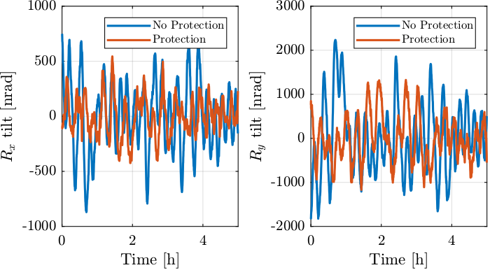
Figure 41: Comparison of the beam angular variations with and without thermal protection

Adding thermal insulator around pillars supporting the optical plates seemed to be a good idea. It indeed lowered the thermal drifts of the temperature of the pillars due to variation of air temperature (Figure 39).

It however did not lower the relative temperature between pillars supporting the same optical plate (Figure 40).

Therefore, it did not improve the tilt motion of the beam due to thermal effects (Figure 41).

6.3. Proposed improvements

There are several ways in which we can improve the stability of the relative motion between the two plates.

6.3.1. Reduce Perturbation

Better Air Conditioning Regulation (i.e. slower variations)
Turn-off the air conditioning during measurement?
Isolate the Laser Setup from the air of the lab. For instance by building an isolated enclosure around the setup.

6.3.2. Reduce Effect of perturbations

Homogenize temperature of all pillars. Could be by building a thermal conductive enclosure around the setup that could help with temperature homogenizing. Could also be by adding thermal bridges between the pillars. However, even if all the pillars have the same temperature, it is possible that there are some Ry and Rz motion when the temperature is varying.
Increase thermal inertia. Supports could be made of granite. Concrete could be added inside the currently used pillars.

6.3.3. Reduce perturbation using feedback control

Active Thermal Control of pillars

6.3.4. Compensation of effect of perturbations

Thermal model of metrology frame and compensation with temperature measurement. The thermal model of the frame could be quite complicated.
Direct measurement of the relative Ry and Rz motion between the two plates. This could be done using an autocollimator or using 3 interferometers.

6.4. Drifts of the metrology plate alone

In order to see if there are some deformations of the optical plate due to thermal drifts, both the laser and the quadrant photodiodes are fixed to the same optical plate.

An exponential fit is performed to remove the long term drifts.

%% Exponential Fit
f = @(b,x) b(1).*exp(b(2).*x) + b(3);

B0 = [3500, -1e-4, 0]; % Initial Estimate

B_Rx = fminsearch(@(b) norm(Rx - f(b,t)), B0);
B_Ry = fminsearch(@(b) norm(Ry - f(b,t)), B0);

The comparison between the measured data and the exponential fit is shown in Figure 42.

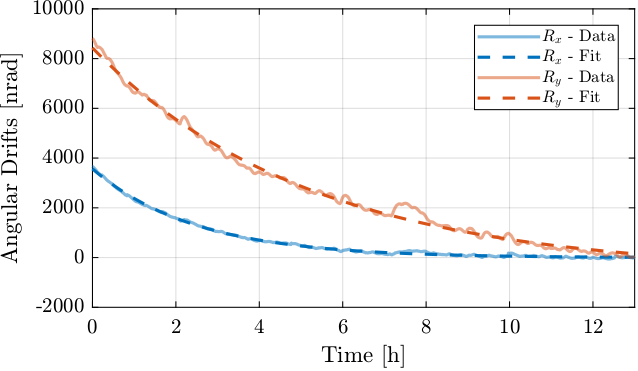
Figure 42: Exponential Fit of the long term thermal drifts

The remaining motion after removing the long term drifts is shown in Figure 43.

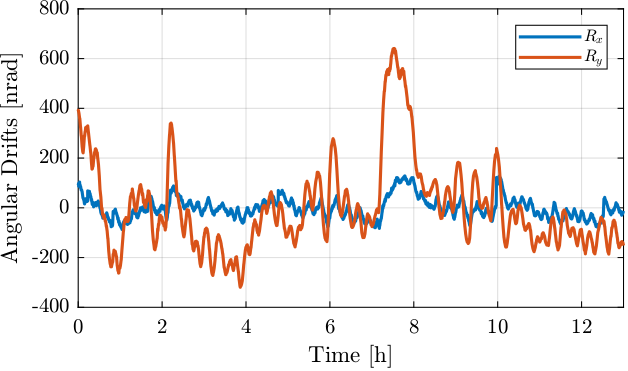
Figure 43: Remaining measured angular drifts after removing the exponential fit

Figure 43 seems to indicate that thermal motion of the pillars supporting the optical plate is inducing some deformation of the optical plate. This is probably due to the fact that the optical plate is mounted on top of the pillars using 3 stiff screws. Using a kinematic mount could help with that regard.

If such deformation is confirmed, this could make the option of measuring the relative motion of the two optical plates with interferometers very complicated to apply.

6.5. Direct measurement of the metrology plate relative motion

In order to separate the angular errors induced by the DCM from the thermal drifts of the optical plates, an external metrology can be added that directly measures the relative motion of the plates, independently of the DCM.

This metrology system must have very small thermal drifts noise.

There are several options:

a similar system than the one used to measured errors of the DCM (i.e. one Laser, a lens and a quadrant photodiode)
an autocollimator
three interferometers

The option studied in this section is the third one using 3 interferometers.

The positions of the interferometers are schematically shown in Figure 44. In such case, the relative angles can be computed from:

\begin{align} d_{R_y} &= \frac{d_C - d_B}{L_{R_y}} \\ d_{R_z} &= \frac{d_A - d_B}{L_{R_z}} \end{align}

interferometer_position_angle_measurement_metrology.png

Figure 44: Figure caption

Increasing the distance between the interferometers (\(L_{R_z}\), \(L_{R_y}\)) permits to have a better sensitivity/lower noise, however the air temperature along the path of the beam may be less homogeneous than if the three interferometers were closer together.

Take an example of \(L_{R_y} = 0.5\,m\). We want the relative stability between the two interferometers to be better than \(25\,nm\) (corresponding to 50 nrad) over 5 minutes and a noise less than \(10\,\text{nrad RMS}\) over a bandwidth of 200Hz.

Regarding noise, the Attocube has a typical noise ASD of \(5 \cdot 10^{-11}\, m/\sqrt{Hz}\). However a bandwidth of 200Hz, this corresponds to \(0.7\,nm\text{ RMS}\) for each Attocube, therefore \(\approx 1\,\text{nm RMS}\) for the differential signal. The two Attocube interferometers should therefore be separated by more than \(10\,cm\) in order to have less than 10 nrad RMS of noise over a bandwidth of 200Hz.

Regarding drifts, as the beam path is quite long (~1.5m), it requires some precautions. We want to have a relative stability better than 25nm over 1.5m (i.e. 0.03ppm). This corresponds to:

relative temperature better than \(15\,mK\)
relative pressure better than \(1.4\,Pa\)
relative humidity better than \(1.5\,\%\)

Clearly, this seems to be hard to achieve if the two beam path are going through separated tubes. Therefore, it is recommended to have the three attocube in the same tube in order to limit the effect of air property variations.

It seems therefore reasonable to have the three Attocube beam path in the same tube with a distance between them of approximately 10 mm.

As a first test, two Attocube are fixed to one optical plate and two corner cubes to the other optical plate.

They are separated by about 50 cm and two plastic tubes are used to limit the air turbulence.

6.5.1. First test - comparison between attocube and photodiodes

The measured data are low pass filtered and the sampling frequency is 1Hz:

Dx, Dy: measured motion of the beam by the quadrant photodiode in nm
Rx, Dy: measured orientation of the beam by the quadrant photodiode in nrad
Rz: measured relative \(R_z\) motion of the two optical plates by the two interferometers, in nrad

On top of that, the temperature of the 8 pillars temp are measured with a sampling frequency of 0.1Hz.

The comparison between the measured \(R_x\) relative angle of the two plates by the photodiode and by the interferometer is done in Figure 45. Even tough the shape of the two measurement is similar, there is a problem of scaling. This could be due to:

wrong identification of the quadrant photodiode gain
problem of relative temperature drifts between the two interferometer beam path
physical effect not understood that induce some relative motion between the interferometers and the laser/photodiode metrology

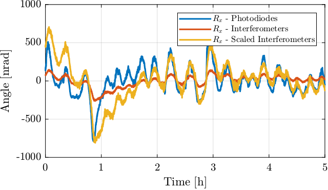
Figure 45: Comparison of the relative Rx angle of the two plates by the photodiode and by the interferometers

This first measurement is not concluding. Additional measurements should be performed in order to determine if this concept of compensating drifts using interferometers could work.

DCM - Laser Setup

Table of Contents

1. Experimental Setup

1.1. Specifications

1.2. Optical Schematic

1.3. Instrumentation

1.3.1. Four Quadrant Photodiode

1.3.2. Transimpedance Amplifier

1.3.3. Analog to Digital Converters

1.3.4. Light Source

1.3.5. XYZ Piezoelectric Stage

2. Alignment of metrology

2.1. Position quadrant photodiode

2.2. Orientation quadrant photodiode

3. Photo-diodes Calibration

3.1. Experimental Setup

3.2. Position 4QD - Calibration

3.3. Orientation 4QD - Calibration

4. Noise Measurement

4.1. ADC Noise

4.2. Noise Coming from long coaxial cables

4.3. Transimpedance Amplifier Noise

4.4. Laser Source Noise

4.5. Mechanical Noise

5. Noise budgeting

5.1. Possible Improvements

5.1.1. Damping of natural frequency

5.1.2. Low pass filtering

5.1.3. Measurement and compensation of high frequency vibrations

6. Stability Measurement

6.1. First Measurement of stability

6.1.1. Measured Beam motion

6.1.2. Measured Temperature

6.1.3. Thermal Model

6.1.4. Comparison of the measured temperature and beam motion

6.1.5. Optimization of temperature compensation

6.2. Measurement with isolated pillars

6.2.1. Measurement with isolated pillars

6.2.2. Evaluation of the benefits of adding thermal insulation

6.3. Proposed improvements

6.3.1. Reduce Perturbation

6.3.2. Reduce Effect of perturbations

6.3.3. Reduce perturbation using feedback control

6.3.4. Compensation of effect of perturbations

6.4. Drifts of the metrology plate alone

6.5. Direct measurement of the metrology plate relative motion

6.5.1. First test - comparison between attocube and photodiodes