Vibration Table
Table of Contents
This report is also available as a pdf.
1 Introduction
This document is divided as follows:
- Section 2: the experimental setup and all the instrumentation are described
- Section 3: the mathematics used to compute the 6DoF motion of a solid body from several inertial sensor is derived
- Section 4: a Simscape model of the vibration table is developed
- Section 6: the table dynamics is identified and compared with the Simscape model
2 Experimental Setup
2.1 CAD Model
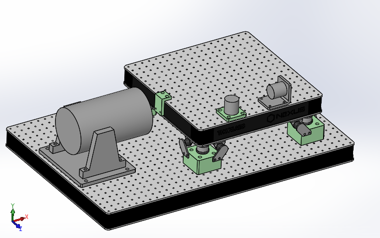
Figure 1: CAD View of the vibration table
2.2 Instrumentation
Here are the documentation of the equipment used for this vibration table:
- Modal Shaker: Watson and Gearing
- Inertial Shaker: IS20
- Viscoelastic supports: 810002
- Spring supports: MV803-12CC
- Optical Table: B4545A
- Triaxial Accelerometer: 356B18
- OROS
2.3 Suspended table
- Dimensions
- 450 mm x 450 mm x 60 mm
- Mass
- 21.30 kg
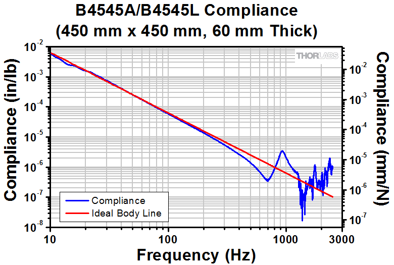
Figure 2: Compliance of the B4545A optical table
If we include including the bottom interface plate:
- Total mass: 30.7 kg
- CoM: 42mm below Center of optical table
- Ix = 0.54, Iy = 0.54, Iz = 1.07 (with respect to CoM)
2.4 Inertial Sensors
| Equipment |
|---|
| (2x) 1D accelerometer PCB 393B05 |
| (4x) 3D accelerometer PCB 356B18 |
3 Compute the 6DoF solid body motion from several inertial sensors
Let’s consider a solid body with several accelerometers attached to it (Figure 3).
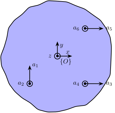
Figure 3: Schematic of the measured motions of a solid body
The goal of this section is to see how to compute the acceleration/angular acceleration of the solid body from the accelerations \(\vec{a}_i\) measured by the accelerometers.
The acceleration/angular acceleration of the solid body is defined as the vector \({}^O\vec{x}\):
\begin{equation} {}^O\vec{x} = \begin{bmatrix} \dot{v}_x \\ \dot{v}_y \\ \dot{v}_z \\ \dot{\omega}_x \\ \dot{\omega}_y \\ \dot{\omega}_z \end{bmatrix} \end{equation}As we want to measure 6dof, we suppose that we have 6 uniaxial acceleremoters (we could use more, but 6 is enough). The measurement of the individual vectors is defined as the vector \(\vec{a}\):
\begin{equation} \vec{a} = \begin{bmatrix} a_1 \\ a_2 \\ a_3 \\ a_4 \\ a_5 \\ a_6 \end{bmatrix} \end{equation}From the positions and orientations of the acceleremoters (defined in Section 3.1), it is quite straightforward to compute the accelerations measured by the sensors from the acceleration/angular acceleration of the solid body (Section 3.2). From this, we can easily build a transformation matrix \(M\), such that:
\begin{equation} \vec{a} = M \cdot {}^O\vec{x} \end{equation}If the matrix is invertible, we can just take the inverse in order to obtain the transformation matrix giving the 6dof acceleration of the solid body from the accelerometer measurements (Section 3.3):
\begin{equation} {}^O\vec{x} = M^{-1} \cdot \vec{a} \end{equation}If it is not invertible, then it means that it is not possible to compute all 6dof of the solid body from the measurements. The solution is then to change the location/orientation of some of the accelerometers.
3.1 Define accelerometers positions/orientations
Let’s first define the position and orientation of all measured accelerations with respect to a defined frame \(\{O\}\).
Opm = [-0.1875, -0.1875, -0.245;
       -0.1875, -0.1875, -0.245;
        0.1875, -0.1875, -0.245;
        0.1875, -0.1875, -0.245;
        0.1875,  0.1875, -0.245;
        0.1875,  0.1875, -0.245]';
There are summarized in Table 1.
| \(a_1\) | \(a_2\) | \(a_3\) | \(a_4\) | \(a_5\) | \(a_6\) | |
|---|---|---|---|---|---|---|
| x | -0.188 | -0.188 | 0.188 | 0.188 | 0.188 | 0.188 |
| y | -0.188 | -0.188 | -0.188 | -0.188 | 0.188 | 0.188 |
| z | -0.245 | -0.245 | -0.245 | -0.245 | -0.245 | -0.245 |
We then define the direction of the measured accelerations (unit vectors):
Osm = [0, 1, 0;
       0, 0, 1;
       1, 0, 0;
       0, 0, 1;
       1, 0, 0;
       0, 1, 0]';
They are summarized in Table 2.
| \(\hat{s}_1\) | \(\hat{s}_2\) | \(\hat{s}_3\) | \(\hat{s}_4\) | \(\hat{s}_5\) | \(\hat{s}_6\) | |
|---|---|---|---|---|---|---|
| x | 0 | 0 | 1 | 0 | 1 | 0 |
| y | 1 | 0 | 0 | 0 | 0 | 0 |
| z | 0 | 1 | 0 | 1 | 0 | 1 |
3.2 Transformation matrix from motion of the solid body to accelerometer measurements
Let’s try to estimate the x-y-z acceleration of any point of the solid body from the acceleration/angular acceleration of the solid body expressed in \(\{O\}\). For any point \(p_i\) of the solid body (corresponding to an accelerometer), we can write:
\begin{equation} \begin{bmatrix} a_{i,x} \\ a_{i,y} \\ a_{i,z} \end{bmatrix} = \begin{bmatrix} \dot{v}_x \\ \dot{v}_y \\ \dot{v}_z \end{bmatrix} + p_i \times \begin{bmatrix} \dot{\omega}_x \\ \dot{\omega}_y \\ \dot{\omega}_z \end{bmatrix} \end{equation}We can write the cross product as a matrix product using the skew-symmetric transformation:
\begin{equation} \begin{bmatrix} a_{i,x} \\ a_{i,y} \\ a_{i,z} \end{bmatrix} = \begin{bmatrix} \dot{v}_x \\ \dot{v}_y \\ \dot{v}_z \end{bmatrix} + \underbrace{\begin{bmatrix} 0 & p_{i,z} & -p_{i,y} \\ -p_{i,z} & 0 & p_{i,x} \\ p_{i,y} & -p_{i,x} & 0 \end{bmatrix}}_{P_{i,[\times]}} \cdot \begin{bmatrix} \dot{\omega}_x \\ \dot{\omega}_y \\ \dot{\omega}_z \end{bmatrix} \end{equation}If we now want to know the (scalar) acceleration \(a_i\) of the point \(p_i\) in the direction of the accelerometer direction \(\hat{s}_i\), we can just project the 3d acceleration on \(\hat{s}_i\):
\begin{equation} a_i = \hat{s}_i^T \cdot \begin{bmatrix} a_{i,x} \\ a_{i,y} \\ a_{i,z} \end{bmatrix} = \hat{s}_i^T \cdot \begin{bmatrix} \dot{v}_x \\ \dot{v}_y \\ \dot{v}_z \end{bmatrix} + \left( \hat{s}_i^T \cdot P_{i,[\times]} \right) \cdot \begin{bmatrix} \dot{\omega}_x \\ \dot{\omega}_y \\ \dot{\omega}_z \end{bmatrix} \end{equation}Which is equivalent as a simple vector multiplication:
\begin{equation} a_i = \begin{bmatrix} \hat{s}_i^T & \hat{s}_i^T \cdot P_{i,[\times]} \end{bmatrix} \begin{bmatrix} \dot{v}_x \\ \dot{v}_y \\ \dot{v}_z \\ \dot{\omega}_x \\ \dot{\omega}_y \\ \dot{\omega}_z \end{bmatrix} = \begin{bmatrix} \hat{s}_i^T & \hat{s}_i^T \cdot P_{i,[\times]} \end{bmatrix} {}^O\vec{x} \end{equation}And finally we can combine the 6 (line) vectors for the 6 accelerometers to write that in a matrix form. We obtain Eq. \eqref{eq:M_matrix}.
The transformation from solid body acceleration \({}^O\vec{x}\) from sensor measured acceleration \(\vec{a}\) is:
\begin{equation} \label{eq:M_matrix} \vec{a} = \underbrace{\begin{bmatrix} \hat{s}_1^T & \hat{s}_1^T \cdot P_{1,[\times]} \\ \vdots & \vdots \\ \hat{s}_6^T & \hat{s}_6^T \cdot P_{6,[\times]} \end{bmatrix}}_{M} {}^O\vec{x} \end{equation}with \(\hat{s}_i\) the unit vector representing the measured direction of the i’th accelerometer expressed in frame \(\{O\}\) and \(P_{i,[\times]}\) the skew-symmetric matrix representing the cross product of the position of the i’th accelerometer expressed in frame \(\{O\}\).
Let’s define such matrix using matlab:
M = zeros(length(Opm), 6);

for i = 1:length(Opm)
    Ri = [0,         Opm(3,i), -Opm(2,i);
         -Opm(3,i),  0,         Opm(1,i);
          Opm(2,i), -Opm(1,i),  0];
    M(i, 1:3) = Osm(:,i)';
    M(i, 4:6) = Osm(:,i)'*Ri;
end
The obtained matrix is shown in Table 3.
| \(\dot{x}_x\) | \(\dot{x}_y\) | \(\dot{x}_z\) | \(\dot{\omega}_x\) | \(\dot{\omega}_y\) | \(\dot{\omega}_z\) | |
|---|---|---|---|---|---|---|
| \(a_1\) | 0.0 | 1.0 | 0.0 | 0.24 | 0.0 | -0.19 |
| \(a_2\) | 0.0 | 0.0 | 1.0 | -0.19 | 0.19 | 0.0 |
| \(a_3\) | 1.0 | 0.0 | 0.0 | 0.0 | -0.24 | 0.19 |
| \(a_4\) | 0.0 | 0.0 | 1.0 | -0.19 | -0.19 | 0.0 |
| \(a_5\) | 1.0 | 0.0 | 0.0 | 0.0 | -0.24 | -0.19 |
| \(a_6\) | 0.0 | 0.0 | 1.0 | 0.19 | -0.19 | 0.0 |
3.3 Compute the transformation matrix from accelerometer measurement to motion of the solid body
In order to compute the motion of the solid body \({}^O\vec{x}\) with respect to frame \(\{O\}\) from the accelerometer measurements \(\vec{a}\), we have to inverse the transformation matrix \(M\).
\begin{equation} {}^O\vec{x} = M^{-1} \vec{a} \end{equation}We therefore need the determinant of \(M\) to be non zero:
det(M)
The obtained inverse of the matrix is shown in Table 4.
| \(a_1\) | \(a_2\) | \(a_3\) | \(a_4\) | \(a_5\) | \(a_6\) | |
|---|---|---|---|---|---|---|
| \(\dot{x}_x\) | 0.0 | 0.7 | 0.5 | -0.7 | 0.5 | 0.0 |
| \(\dot{x}_y\) | 1.0 | 0.0 | 0.5 | 0.7 | -0.5 | -0.7 |
| \(\dot{x}_z\) | 0.0 | 0.5 | 0.0 | 0.0 | 0.0 | 0.5 |
| \(\dot{\omega}_x\) | 0.0 | 0.0 | 0.0 | -2.7 | 0.0 | 2.7 |
| \(\dot{\omega}_y\) | 0.0 | 2.7 | 0.0 | -2.7 | 0.0 | 0.0 |
| \(\dot{\omega}_z\) | 0.0 | 0.0 | 2.7 | 0.0 | -2.7 | 0.0 |
4 Simscape Model
In this section, the Simscape model of the vibration table is described.
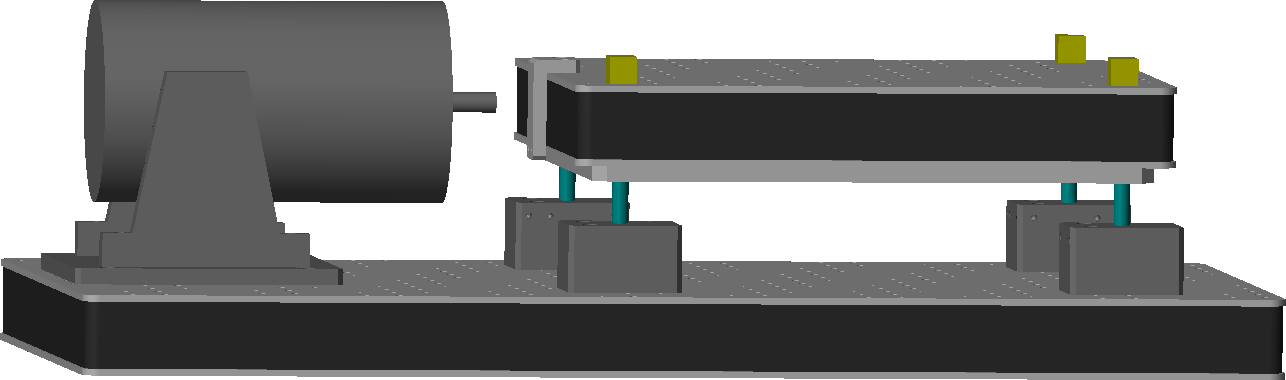
Figure 4: 3D representation of the simscape model
4.1 Simscape Sub-systems
4.1.1 Springs
The 4 springs supporting the suspended optical table are modelled with “bushing joints” having stiffness and damping in the x-y-z directions:
spring.kx = 1e4; % X- Stiffness [N/m]
spring.cx = 1e1; % X- Damping [N/(m/s)]

spring.ky = 1e4; % Y- Stiffness [N/m]
spring.cy = 1e1; % Y- Damping [N/(m/s)]

spring.kz = 1e4; % Z- Stiffness [N/m]
spring.cz = 1e1; % Z- Damping [N/(m/s)]

spring.z0 = 32e-3; % Equilibrium z-length [m]
And we can increase the “equilibrium position” of the vertical springs to take into account the gravity forces and start closer to equilibrium:
spring.dl = (30.5918/4)*9.80665/spring.kz;
4.1.2 Inertial Shaker (IS20)
The inertial shaker is defined as two solid bodies:
- the “housing” that is fixed to the element that we want to excite
- the “inertial mass” that is suspended inside the housing
The inertial mass is guided inside the housing and an actuator (coil and magnet) can be used to apply a force between the inertial mass and the support. The “reacting” force on the support is then used as an excitation.
| Characteristic | Value |
|---|---|
| Output Force | 20 N |
| Frequency Range | 10-3000 Hz |
| Moving Mass | 0.1 kg |
| Total Mass | 0.3 kg |
From the datasheet in Table 5, we can estimate the parameters of the physical shaker.
These parameters are defined below
shaker.w0 = 2*pi*10; % Resonance frequency of moving mass [rad/s]
shaker.m = 0.1; % Moving mass [m]
shaker.m_tot = 0.3; % Total mass [m]
shaker.k = shaker.m*shaker.w0^2; % Spring constant [N/m]
shaker.c = 0.2*sqrt(shaker.k*shaker.m); % Damping [N/(m/s)]
4.1.3 3D accelerometer (356B18)
An accelerometer consists of 2 solids:
- a “housing” rigidly fixed to the measured body
- an “inertial mass” suspended inside the housing by springs and guided in the measured direction
The relative motion between the housing and the inertial mass gives a measurement of the acceleration of the measured body (up to the suspension mode of the inertial mass).
| Characteristic | Value |
|---|---|
| Sensitivity | 0.102 V/(m/s2) |
| Frequency Range | 0.5 to 3000 Hz |
| Resonance Frequency | > 20 kHz |
| Resolution | 0.0005 m/s2 rms |
| Weight | 0.025 kg |
| Size | 20.3x26.1x20.3 [mm] |
Here are defined the parameters for the triaxial accelerometer:
acc_3d.m = 0.005; % Inertial mass [kg]
acc_3d.m_tot = 0.025; % Total mass [m]

acc_3d.w0 = 2*pi*20e3; % Resonance frequency [rad/s]

acc_3d.kx = acc_3d.m*acc_3d.w0^2; % Spring constant [N/m]
acc_3d.ky = acc_3d.m*acc_3d.w0^2; % Spring constant [N/m]
acc_3d.kz = acc_3d.m*acc_3d.w0^2; % Spring constant [N/m]

acc_3d.cx = 1e2; % Damping [N/(m/s)]
acc_3d.cy = 1e2; % Damping [N/(m/s)]
acc_3d.cz = 1e2; % Damping [N/(m/s)]
DC gain between support acceleration and inertial mass displacement is \(-m/k\):
acc_3d.g_x = 1/(-acc_3d.m/acc_3d.kx); % [m/s^2/m]
acc_3d.g_y = 1/(-acc_3d.m/acc_3d.ky); % [m/s^2/m]
acc_3d.g_z = 1/(-acc_3d.m/acc_3d.kz); % [m/s^2/m]
We also define the sensitivity in order to have the outputs in volts.
acc_3d.gV_x = 0.102; % [V/(m/s^2)]
acc_3d.gV_y = 0.102; % [V/(m/s^2)]
acc_3d.gV_z = 0.102; % [V/(m/s^2)]
The problem with using such model for accelerometers is that this adds states to the identified models (2x3 states for each triaxial accelerometer). These states represents the dynamics of the suspended inertial mass. In the frequency band of interest (few Hz up to ~1 kHz), the dynamics of the inertial mass can be ignore (its resonance is way above 1kHz). Therefore, we might as well use idealized “transform sensors” blocks as they will give the same result up to ~20kHz while allowing to reduce the number of identified states.
The accelerometer model can be chosen by setting the type property:
acc_3d.type = 2; % 1: inertial mass, 2: perfect
4.2 Identification
4.2.1 Number of states
Let’s first use perfect 3d accelerometers:
acc_3d.type = 2; % 1: inertial mass, 2: perfect
And identify the dynamics from the shaker force to the measured accelerations:
%% Name of the Simulink File
mdl = 'vibration_table';

%% Input/Output definition
clear io; io_i = 1;
io(io_i) = linio([mdl, '/F'],  1, 'openinput');  io_i = io_i + 1;
io(io_i) = linio([mdl, '/acc'],  1, 'openoutput'); io_i = io_i + 1;

%% Run the linearization
Gp = linearize(mdl, io);
Gp.InputName  = {'F'};
Gp.OutputName  = {'a1', 'a2', 'a3', 'a4', 'a5', 'a6'};
size(Gp)
State-space model with 6 outputs, 1 inputs, and 12 states.
We indeed have the 12 states corresponding to the 6 DoF of the suspended optical table.
Let’s now consider the inertial masses for the triaxial accelerometers:
acc_3d.type = 1; % 1: inertial mass, 2: perfect
%% Name of the Simulink File
mdl = 'vibration_table';

%% Input/Output definition
clear io; io_i = 1;
io(io_i) = linio([mdl, '/F'],  1, 'openinput');  io_i = io_i + 1;
io(io_i) = linio([mdl, '/acc'],  1, 'openoutput'); io_i = io_i + 1;

%% Run the linearization
Ga = linearize(mdl, io);
Ga.InputName  = {'F'};
Ga.OutputName  = {'a1', 'a2', 'a3', 'a4', 'a5', 'a6'};
size(Ga)
State-space model with 6 outputs, 1 inputs, and 30 states.
And we can see that 18 states have been added. This corresponds to 6 states for each triaxial accelerometers.
4.2.2 Resonance frequencies and mode shapes
Let’s now identify the resonance frequency and mode shapes associated with the suspension modes of the optical table.
acc_3d.type = 2; % 1: inertial mass, 2: perfect

%% Name of the Simulink File
mdl = 'vibration_table';

%% Input/Output definition
clear io; io_i = 1;
io(io_i) = linio([mdl, '/F'],      1, 'openinput');  io_i = io_i + 1;
io(io_i) = linio([mdl, '/a1,a2'],  1, 'openoutput'); io_i = io_i + 1;

%% Run the linearization
G = linearize(mdl, io);
G.InputName  = {'F'};
G.OutputName  = {'ax'};
Compute the resonance frequencies
ws = eig(G.A);
ws = ws(imag(ws) > 0);
And the associated response of the optical table
x_mod = zeros(6, 6);

for i = 1:length(ws)
    xi = evalfr(G, ws(i));
    x_mod(:,i) = xi./norm(xi);
end
The results are shown in Table 7. The motion associated to the mode shapes are just indicative.
| \(\omega_0\) [Hz] | 5.6 | 5.6 | 5.7 | 8.2 | 8.2 | 8.2 |
|---|---|---|---|---|---|---|
| x | 0.1 | 0.7 | 0.0 | 0.0 | 0.2 | 0.0 |
| y | 0.7 | 0.1 | 0.0 | 0.0 | 0.0 | 0.2 |
| z | 0.0 | 0.0 | 1.0 | 0.0 | 0.0 | 0.0 |
| Rx | 0.7 | 0.1 | 0.0 | 0.0 | 0.1 | 1.0 |
| Ry | 0.1 | 0.7 | 0.0 | 0.0 | 1.0 | 0.1 |
| Rz | 0.0 | 0.0 | 0.0 | 1.0 | 0.0 | 0.0 |
4.3 Verify transformation
%% Options for Linearized
options = linearizeOptions;
options.SampleTime = 0;

%% Name of the Simulink File
mdl = 'vibration_table';

%% Input/Output definition
clear io; io_i = 1;
io(io_i) = linio([mdl, '/F'],  1, 'openinput');  io_i = io_i + 1;
io(io_i) = linio([mdl, '/acc'],  1, 'openoutput'); io_i = io_i + 1;
io(io_i) = linio([mdl, '/acc_O'],  1, 'openoutput'); io_i = io_i + 1;

%% Run the linearization
G = linearize(mdl, io, 0.0, options);
G.InputName  = {'F'};
G.OutputName = {'a1', 'a2', 'a3', 'a4', 'a5', 'a6', ...
                'Dx', 'Dy', 'Dz', 'Rx', 'Ry', 'Rz'};
G_acc = inv(M)*G(1:6, 1);
G_id = G(7:12, 1);
bodeFig({G_acc(1), G_id(1)})
bodeFig({G_acc(2), G_id(2)})
bodeFig({G_acc(3), G_id(3)})
bodeFig({G_acc(4), G_id(4)})
bodeFig({G_acc(5), G_id(5)})
bodeFig({G_acc(6), G_id(6)})
5 Nano-Hexapod
A configuration is added to be able to put the nano-hexapod on top of the vibration table as shown in Figure 4.
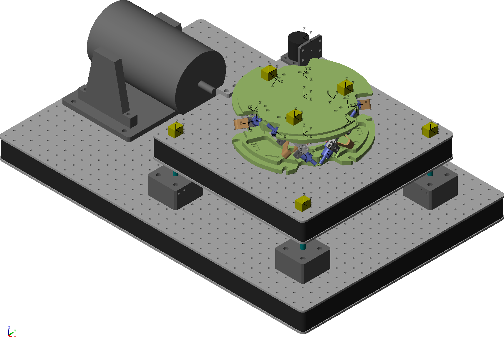
Figure 5: 3D representation of the simscape model with the nano-hexapod
The nano-hexapod’s simscape model is taken from another git repository.
5.1 Nano-Hexapod
n_hexapod = initializeNanoHexapodFinal('flex_bot_type', '4dof', ...
                                       'flex_top_type', '3dof', ...
                                       'motion_sensor_type', 'struts', ...
                                       'actuator_type', '2dof');
5.2 Computation of the transmissibility from accelerometer data
The goal is to compute the \(6 \times 6\) transfer function matrix corresponding to the transmissibility of the Nano-Hexapod.
To do so, several accelerometers are located both on the vibration table and on the top of the nano-hexapod.
The vibration table is then excited using a Shaker and all the accelerometers signals are recorded.
Using transformation (jacobian) matrices, it is then possible to compute both the motion of the top and bottom platform of the nano-hexapod.
Finally, it is possible to compute the \(6 \times 6\) transmissibility matrix.
Such procedure is explained in (Marneffe and André 2004).
5.2.1 Jacobian matrices
How to compute the Jacobian matrices is explained in Section 3.
%% Bottom Accelerometers
Opb = [-0.1875, -0.1875, -0.245;
       -0.1875, -0.1875, -0.245;
        0.1875, -0.1875, -0.245;
        0.1875, -0.1875, -0.245;
        0.1875,  0.1875, -0.245;
        0.1875,  0.1875, -0.245]';

Osb = [0, 1, 0;
       0, 0, 1;
       1, 0, 0;
       0, 0, 1;
       1, 0, 0;
       0, 0, 1;]';

Jb = zeros(length(Opb), 6);

for i = 1:length(Opb)
    Ri = [0,         Opb(3,i), -Opb(2,i);
         -Opb(3,i),  0,         Opb(1,i);
          Opb(2,i), -Opb(1,i),  0];
    Jb(i, 1:3) = Osb(:,i)';
    Jb(i, 4:6) = Osb(:,i)'*Ri;
end

Jbinv = inv(Jb);
| \(a_1\) | \(a_2\) | \(a_3\) | \(a_4\) | \(a_5\) | \(a_6\) | |
|---|---|---|---|---|---|---|
| \(\dot{x}_x\) | 0.0 | 0.7 | 0.5 | -0.7 | 0.5 | 0.0 |
| \(\dot{x}_y\) | 1.0 | 0.0 | 0.5 | 0.7 | -0.5 | -0.7 |
| \(\dot{x}_z\) | 0.0 | 0.5 | 0.0 | 0.0 | 0.0 | 0.5 |
| \(\dot{\omega}_x\) | 0.0 | 0.0 | 0.0 | -2.7 | 0.0 | 2.7 |
| \(\dot{\omega}_y\) | 0.0 | 2.7 | 0.0 | -2.7 | 0.0 | 0.0 |
| \(\dot{\omega}_z\) | 0.0 | 0.0 | 2.7 | 0.0 | -2.7 | 0.0 |
%% Top Accelerometers
Opt = [-0.1,   0,     -0.150;
       -0.1,   0,     -0.150;
        0.05,  0.075, -0.150;
        0.05,  0.075, -0.150;
        0.05, -0.075, -0.150;
        0.05, -0.075, -0.150]';

Ost = [0, 1, 0;
       0, 0, 1;
       1, 0, 0;
       0, 0, 1;
       1, 0, 0;
       0, 0, 1;]';

Jt = zeros(length(Opt), 6);

for i = 1:length(Opt)
    Ri = [0,         Opt(3,i), -Opt(2,i);
         -Opt(3,i),  0,         Opt(1,i);
          Opt(2,i), -Opt(1,i),  0];
    Jt(i, 1:3) = Ost(:,i)';
    Jt(i, 4:6) = Ost(:,i)'*Ri;
end

Jtinv = inv(Jt);
| \(b_1\) | \(b_2\) | \(b_3\) | \(b_4\) | \(b_5\) | \(b_6\) | |
|---|---|---|---|---|---|---|
| \(\dot{x}_x\) | 0.0 | 1.0 | 0.5 | -0.5 | 0.5 | -0.5 |
| \(\dot{x}_y\) | 1.0 | 0.0 | -0.7 | -1.0 | 0.7 | 1.0 |
| \(\dot{x}_z\) | 0.0 | 0.3 | 0.0 | 0.3 | 0.0 | 0.3 |
| \(\dot{\omega}_x\) | 0.0 | 0.0 | 0.0 | 6.7 | 0.0 | -6.7 |
| \(\dot{\omega}_y\) | 0.0 | 6.7 | 0.0 | -3.3 | 0.0 | -3.3 |
| \(\dot{\omega}_z\) | 0.0 | 0.0 | -6.7 | 0.0 | 6.7 | 0.0 |
5.2.2 Using linearize function
acc_3d.type = 2; % 1: inertial mass, 2: perfect

%% Name of the Simulink File
mdl = 'vibration_table';

%% Input/Output definition
clear io; io_i = 1;
io(io_i) = linio([mdl, '/F_shaker'], 1, 'openinput');  io_i = io_i + 1;
io(io_i) = linio([mdl, '/acc'],      1, 'openoutput'); io_i = io_i + 1;
io(io_i) = linio([mdl, '/acc_top'],  1, 'openoutput'); io_i = io_i + 1;

%% Run the linearization
G = linearize(mdl, io);
G.InputName  = {'F1', 'F2', 'F3', 'F4', 'F5', 'F6'};
G.OutputName  = {'a1', 'a2', 'a3', 'a4', 'a5', 'a6', ...
                 'b1', 'b2', 'b3', 'b4', 'b5', 'b6'};
Gb = Jbinv*G({'a1', 'a2', 'a3', 'a4', 'a5', 'a6'}, :);
Gt = Jtinv*G({'b1', 'b2', 'b3', 'b4', 'b5', 'b6'}, :);
T = inv(Gb)*Gt;
T = minreal(T);
T = prescale(T, {2*pi*0.1, 2*pi*1e3});
5.3 Comparison with “true” transmissibility
%% Name of the Simulink File
mdl = 'test_transmissibility';

%% Input/Output definition
clear io; io_i = 1;
io(io_i) = linio([mdl, '/d'],   1, 'openinput');  io_i = io_i + 1;
io(io_i) = linio([mdl, '/acc'], 1, 'openoutput'); io_i = io_i + 1;

%% Run the linearization
G = linearize(mdl, io);
G.InputName  = {'Dx', 'Dy', 'Dz', 'Rx', 'Ry', 'Rz'};
G.OutputName  = {'Ax', 'Ay', 'Az', 'Bx', 'By', 'Bz'};
Tp = G/s^2;
6 Identification of the table’s dynamics
6.1 Mode Shapes
| Freq. [Hz] | Description | |
|---|---|---|
| 1 | 1.3 | X-translation |
| 2 | 1.3 | Y-translation |
| 3 | 1.95 | Z-rotation |
| 4 | 6.85 | Z-translation |
| 5 | 8.9 | Tilt |
| 6 | 8.9 | Tilt |
| 7 | 700 | Flexible Mode |
Figure 6: Mode shapes of the 6 suspension modes (from 1Hz to 9Hz)
Figure 7: First flexible mode of the table at 700Hz