Flexible Joints - Test Bench
Table of Contents
- 1. Flexible Joints
- 2. Dimensional Measurements
- 3. Measurement Test Bench - Bending Stiffness
- 4. Error budget
- 4.1. Finite Element Model
- 4.2. Setup
- 4.3. Effect of Bending
- 4.4. Computation of the bending stiffness
- 4.5. Estimation error due to force and displacement sensors accuracy
- 4.6. Estimation error due to Shear
- 4.7. Estimation error due to force sensor compression
- 4.8. Estimation error due to height estimation error
- 4.9. Conclusion
- 5. First Measurements
- 6. Bending Stiffness Measurement
This report is also available as a pdf.
In this document, we present a test-bench that has been developed in order to measure the bending stiffness of flexible joints.
It is structured as follow:
- Section 1: the geometry of the flexible joints and the expected stiffness and stroke are presented
- Section 2: each flexible joint is measured using a profile projector
- Section 3: the stiffness measurement bench is presented
- Section 4: an error budget is performed in order to estimate the accuracy of the measured stiffness
- Section 5: first measurements are performed
- Section 6: the bending stiffness of the flexible joints are measured
1 Flexible Joints
The flexible joints that are going to be measured in this document have been design to be used with a Nano-Hexapod (Figure 1).
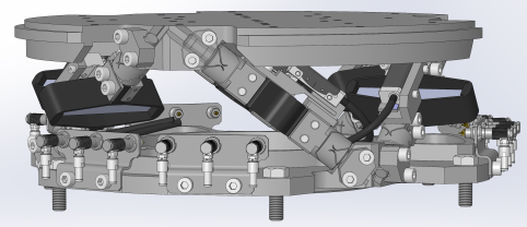
Figure 1: CAD view of the Nano-Hexapod containing the flexible joints
Ideally, these flexible joints would behave as perfect ball joints, that is to say:
- no bending and torsional stiffnesses
- infinite shear and axial stiffnesses
- un-limited bending and torsional stroke
- no friction, no backlash
The real characteristics of the flexible joints will influence the dynamics of the Nano-Hexapod. Using a multi-body dynamical model of the nano-hexapod, the specifications in term of stiffness and stroke of the flexible joints have been determined and summarized in Table 1.
| Specification | FEM | |
|---|---|---|
| Axial Stiffness | > 100 [N/um] | 94 |
| Shear Stiffness | > 1 [N/um] | 13 |
| Bending Stiffness | < 100 [Nm/rad] | 5 |
| Torsion Stiffness | < 500 [Nm/rad] | 260 |
| Bending Stroke | > 1 [mrad] | 24.5 |
| Torsion Stroke | > 5 [urad] |
Then, the classical geometry of a flexible ball joint shown in Figure 2 has been optimized in order to meet the requirements. This has been done using a Finite Element Software and the obtained joint’s characteristics are summarized in Table 1.
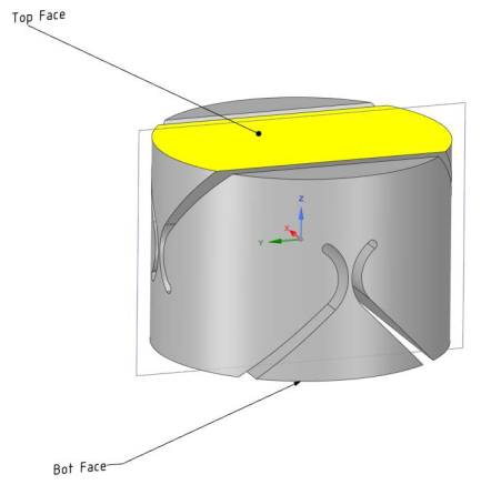
Figure 2: Flexible part of the Joint used for FEM - CAD view
The obtained geometry are defined in the drawings of the flexible joints. The material is a special kind of stainless steel called “F16PH”.
The flexible joints can be seen on Figure 3.
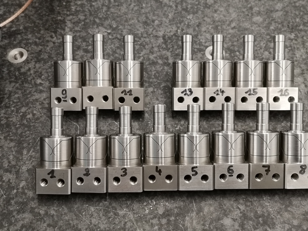
Figure 3: 15 of the 16 flexible joints
2 Dimensional Measurements
2.1 Measurement Bench
The axis corresponding to the flexible joints are defined in Figure 4.

Figure 4: Define axis for the flexible joints
The dimensions of the flexible part in the Y-Z plane will contribute to the X-bending stiffness. Similarly, the dimensions of the flexible part in the X-Z plane will contribute to the Y-bending stiffness.
The setup to measure the dimension of the “X” flexible beam is shown in Figure 5.
Figure 5: Setup to measure the dimension of the flexible beam corresponding to the X-bending stiffness
What we typically observe is shown in Figure 6. It is then possible to estimate to dimension of the flexible beam with an accuracy of \(\approx 5\,\mu m\),
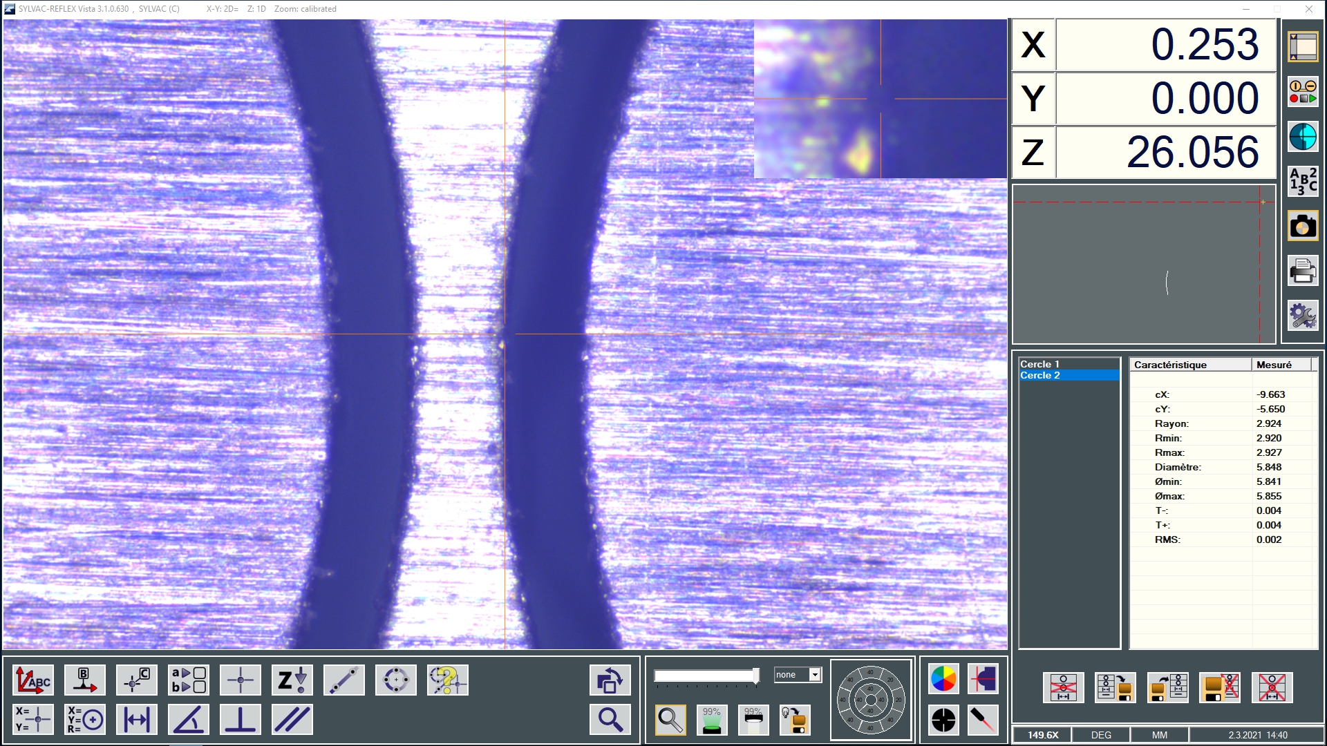
Figure 6: Image used to measure the flexible joint’s dimensions
2.2 Measurement Results
The expected flexible beam thickness is \(250\,\mu m\). However, it is more important that the thickness of all beams are close to each other.
The dimension of the beams are been measured at each end to be able to estimate the mean of the beam thickness.
All the measured dimensions are summarized in Table 2.
| Y1 | Y2 | X1 | X2 | |
|---|---|---|---|---|
| 1 | 223 | 226 | 224 | 214 |
| 2 | 229 | 231 | 237 | 224 |
| 3 | 234 | 230 | 239 | 231 |
| 4 | 233 | 227 | 229 | 232 |
| 5 | 225 | 212 | 228 | 228 |
| 6 | 220 | 221 | 224 | 220 |
| 7 | 206 | 207 | 228 | 226 |
| 8 | 230 | 224 | 224 | 223 |
| 9 | 223 | 231 | 228 | 233 |
| 10 | 228 | 230 | 235 | 231 |
| 11 | 197 | 207 | 211 | 204 |
| 12 | 227 | 226 | 225 | 226 |
| 13 | 215 | 228 | 231 | 220 |
| 14 | 216 | 224 | 224 | 221 |
| 15 | 209 | 214 | 220 | 221 |
| 16 | 213 | 210 | 230 | 229 |
An histogram of these measured dimensions is shown in Figure 7.
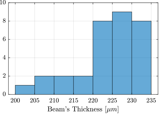
Figure 7: Histogram for the (16x2) measured beams’ thickness
3 Measurement Test Bench - Bending Stiffness
The most important characteristic of the flexible joint that we want to measure is its bending stiffness \(k_{R_x} \approx k_{R_y}\).
To do so, we have to apply a torque \(T_x\) on the flexible joint and measure its angular deflection \(\theta_x\). The stiffness is then
\begin{equation} k_{R_x} = \frac{T_x}{\theta_x} \end{equation}As it is quite difficult to apply a pure torque, a force will be applied instead. The application point of the force should far enough from the flexible part such that the obtained bending is much larger than the displacement in shear.
The working principle of the bench is schematically shown in Figure 8. One part of the flexible joint is fixed. On the mobile part, a force \(F_x\) is applied which is equivalent to a torque applied on the flexible joint center. The induced rotation is measured with a displacement sensor \(d_x\).
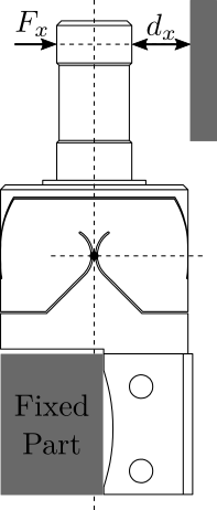
Figure 8: Test Bench - working principle
This test-bench will be used to have a first approximation of the bending stiffnesss and stroke of the flexible joints. Another test-bench, better engineered will be used to measure the flexible joint’s characteristics with better accuracy.
3.1 Flexible joint Geometry
The flexible joint used for the Nano-Hexapod is shown in Figure 9. Its bending stiffness is foreseen to be \(k_{R_y}\approx 5\,\frac{Nm}{rad}\) and its stroke \(\theta_{y,\text{max}}\approx 25\,mrad\).

Figure 9: Geometry of the flexible joint
The height between the flexible point (center of the joint) and the point where external forces are applied is \(h = 20\,mm\).
Let’s define the parameters on Matlab.
kRx = 5; % Bending Stiffness [Nm/rad]
Rxmax = 25e-3; % Bending Stroke [rad]
h = 20e-3; % Height [m]
3.2 Required external applied force
The bending \(\theta_y\) of the flexible joint due to the force \(F_x\) is:
\begin{equation} \theta_y = \frac{M_y}{k_{R_y}} = \frac{F_x h}{k_{R_y}} \end{equation}Therefore, the applied force to test the full range of the flexible joint is:
\begin{equation} F_{x,\text{max}} = \frac{k_{R_y} \theta_{y,\text{max}}}{h} \end{equation}Fxmax = kRx*Rxmax/h; % Force to induce maximum stroke [N]
And we obtain:
\begin{equation} F_{x,max} = 6.2\, [N] \end{equation}The measurement range of the force sensor should then be higher than \(6.2\,N\).
3.3 Required actuator stroke and sensors range
The flexible joint is designed to allow a bending motion of \(\pm 25\,mrad\). The corresponding stroke at the location of the force sensor is: \[ d_{x,\text{max}} = h \tan(R_{x,\text{max}}) \]
dxmax = h*tan(Rxmax);
In order to test the full range of the flexible joint, the stroke of the translation stage used to move the force sensor should be higher than \(0.5\,mm\). Similarly, the measurement range of the displacement sensor should also be higher than \(0.5\,mm\).
3.4 Test Bench
A CAD view of the measurement bench is shown in Figure 10.
Here are the different elements used in this bench:
- Translation Stage: V-408
- Load Cells: FC2231-0000-0010-L
- Encoder: Renishaw Resolute 1nm
Both the measured force and displacement are acquired at the same time using a Speedgoat machine.
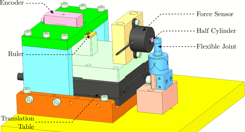
Figure 10: Schematic of the test bench to measure the bending stiffness of the flexible joints
A side view of the bench with the important quantities are shown in Figure 11.
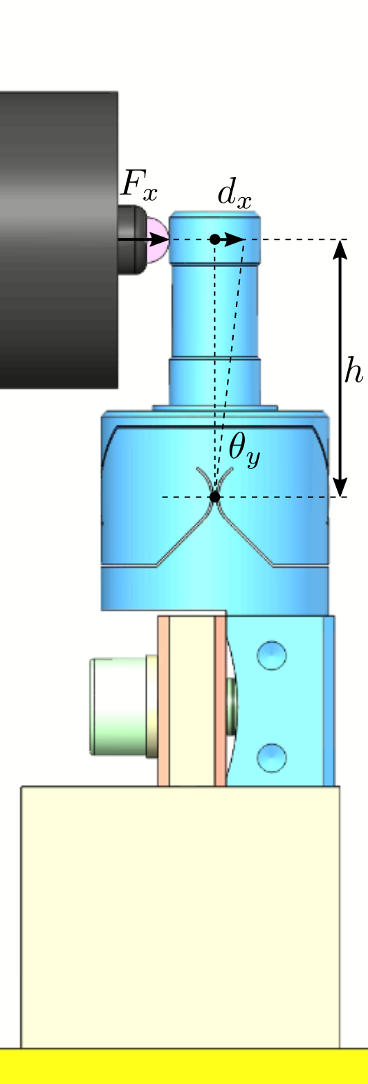
Figure 11: Schematic of the test bench to measure the bending stiffness of the flexible joints
4 Error budget
Many things can impact the accuracy of the measured bending stiffness such as:
- Errors in the force and displacement measurement
- Shear effects
- Deflection of the Force sensor
- Errors in the geometry of the bench
In this section, we wish to estimate the attainable accuracy with the current bench, and identified the limiting factors.
4.1 Finite Element Model
From the Finite Element Model, the stiffness and stroke of the flexible joint have been computed and summarized in Tables 3 and 4.
| Stiffness [N/um] | Max Force [N] | Stroke [um] | |
|---|---|---|---|
| Axial | 94 | 469 | 5 |
| Shear | 13 | 242 | 19 |
| Stiffness [Nm/rad] | Max Torque [Nmm] | Stroke [mrad] | |
|---|---|---|---|
| Bending | 5 | 118 | 24 |
| Torsional | 260 | 1508 | 6 |
4.2 Setup
The setup is schematically represented in Figure 12.
The force is applied on top of the flexible joint with a distance \(h\) with the joint’s center. The displacement of the flexible joint is also measured at the same height.
The height between the joint’s center and the force application point is:
h = 25e-3; % Height [m]
Figure 12: Schematic of the test bench to measure the bending stiffness of the flexible joints
4.3 Effect of Bending
The torque applied is:
\begin{equation} M_y = F_x \cdot h \end{equation}The flexible joint is experiencing a rotation \(\theta_y\) due to the torque \(M_y\):
\begin{equation} \theta_y = \frac{M_y}{k_{R_y}} = \frac{F_x \cdot h}{k_{R_y}} \end{equation}This rotation is then measured by the displacement sensor. The measured displacement is:
\begin{equation} D_b = h \tan(\theta_y) = h \tan\left( \frac{F_x \cdot h}{k_{R_y}} \right) \label{eq:bending_stiffness_formula} \end{equation}4.4 Computation of the bending stiffness
From equation \eqref{eq:bending_stiffness_formula}, we can compute the bending stiffness:
\begin{equation} k_{R_y} = \frac{F_x \cdot h}{\tan^{-1}\left( \frac{D_b}{h} \right)} \end{equation}For small displacement, we have
\begin{equation} \boxed{k_{R_y} \approx h^2 \frac{F_x}{d_x}} \end{equation}And therefore, to precisely measure \(k_{R_y}\), we need to:
- precisely measure the motion \(d_x\)
- precisely measure the applied force \(F_x\)
- precisely now the height of the force application point \(h\)
4.5 Estimation error due to force and displacement sensors accuracy
The maximum error on the measured displacement with the encoder is 40 nm. This quite negligible compared to the measurement range of 0.5 mm.
The accuracy of the force sensor is around 1% and therefore, we should expect to have an accuracy on the measured stiffness of at most 1%.
4.6 Estimation error due to Shear
The effect of Shear on the measured displacement is simply:
\begin{equation} D_s = \frac{F_x}{k_s} \end{equation}The measured displacement will be the effect of shear + effect of bending
\begin{equation} d_x = D_b + D_s = h \tan\left( \frac{F_x \cdot h}{k_{R_y}} \right) + \frac{F_x}{k_s} \approx F_x \left( \frac{h^2}{k_{R_y}} + \frac{1}{k_s} \right) \end{equation}The estimated bending stiffness \(k_{\text{est}}\) will then be:
\begin{equation} k_{\text{est}} = h^2 \frac{F_x}{d_x} \approx k_{R_y} \frac{1}{1 + \frac{k_{R_y}}{k_s h^2}} \end{equation}The measurement error due to Shear is 0.1 %
4.7 Estimation error due to force sensor compression
The measured displacement is not done directly at the joint’s location. The force sensor compression will then induce an error on the joint’s stiffness.
The force sensor stiffness \(k_F\) is estimated to be around:
kF = 50/0.05e-3; % [N/m]
k_F = 1.0e+06 [N/m]
The measured displacement will be the sum of the displacement induced by the bending and by the compression of the force sensor:
\begin{equation} d_x = D_b + \frac{F_x}{k_F} = h \tan\left( \frac{F_x \cdot h}{k_{R_y}} \right) + \frac{F_x}{k_F} \approx F_x \left( \frac{h^2}{k_{R_y}} + \frac{1}{k_F} \right) \end{equation}The estimated bending stiffness \(k_{\text{est}}\) will then be:
\begin{equation} k_{\text{est}} = h^2 \frac{F_x}{d_x} \approx k_{R_y} \frac{1}{1 + \frac{k_{R_y}}{k_F h^2}} \end{equation}The measurement error due to height estimation errors is 0.8 %
4.8 Estimation error due to height estimation error
Let’s consider an error in the estimation of the height from the application of the force to the joint’s center:
\begin{equation} h_{\text{est}} = h (1 + \epsilon) \end{equation}The computed bending stiffness will be:
\begin{equation} k_\text{est} \approx h_{\text{est}}^2 \frac{F_x}{d_x} \end{equation}And the stiffness estimation error is:
\begin{equation} \frac{k_{\text{est}}}{k_{R_y}} = (1 + \epsilon)^2 \end{equation}h_err = 0.2e-3; % Height estimation error [m]
The measurement error due to height estimation errors of 0.2 [mm] is 1.6 %
4.9 Conclusion
Based on the above analysis, we should expect no better than few percent of accuracy using the current test-bench. This is well enough for a first estimation of the bending stiffness of the flexible joints.
Another measurement bench allowing better accuracy will be developed.
5 First Measurements
5.1 Agreement between the probe and the encoder
- Encoder: Renishaw Resolute 1nm
- Displacement Probe: Millimar C1216 electronics and Millimar 1318 probe
The measurement setup is made such that the probe measured the translation table displacement. It should then measure the same displacement as the encoder. Using this setup, we should be able to compare the probe and the encoder.
Let’s load the measurements.
load('meas_probe_against_encoder.mat', 't', 'd', 'dp', 'F')
The time domain measured displacement by the probe and by the encoder is shown in Figure 13.
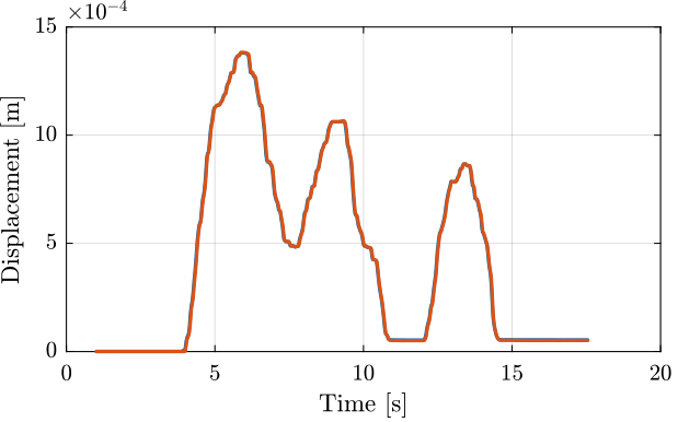
Figure 13: Time domain measurement
If we zoom, we see that there is some delay between the encoder and the probe (Figure 14).
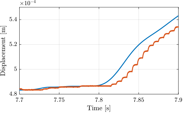
Figure 14: Time domain measurement (Zoom)
This delay is estimated using the finddelay command.
The time delay is approximately 15.8 [ms]
The measured mismatch between the encoder and the probe with and without compensating for the time delay are shown in Figure 15.
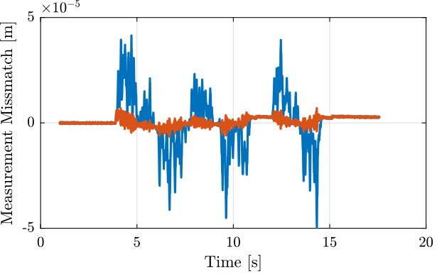
Figure 15: Measurement mismatch, with and without delay compensation
Finally, the displacement of the probe is shown as a function of the displacement of the encoder and a linear fit is made (Figure 16).
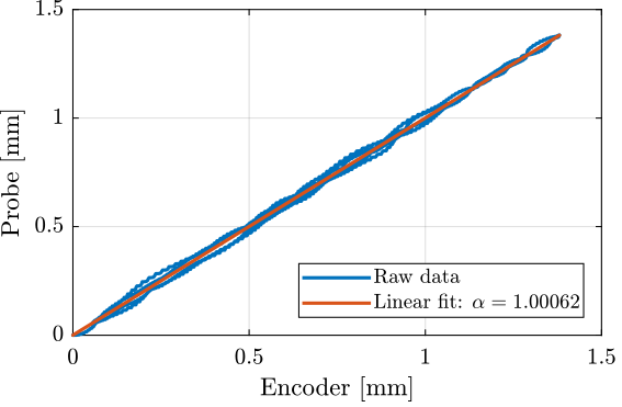
Figure 16: Measured displacement by the probe as a function of the measured displacement by the encoder
From the measurement, it is shown that the probe is well calibrated. However, there is some time delay of tens of milliseconds that could induce some measurement errors.
5.2 Measurement of the Millimar 1318 probe stiffness
- Translation Stage: V-408
- Load Cell: FC2231-0000-0010-L
- Encoder: Renishaw Resolute 1nm
- Displacement Probe: Millimar C1216 electronics and Millimar 1318 probe
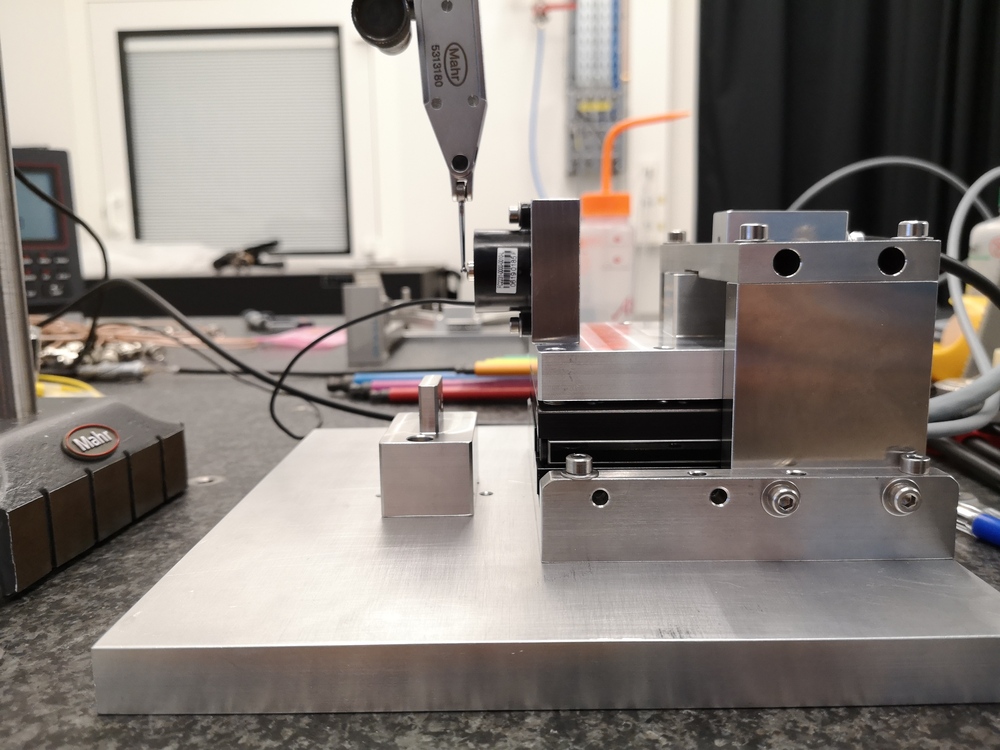
Figure 17: Setup - Side View
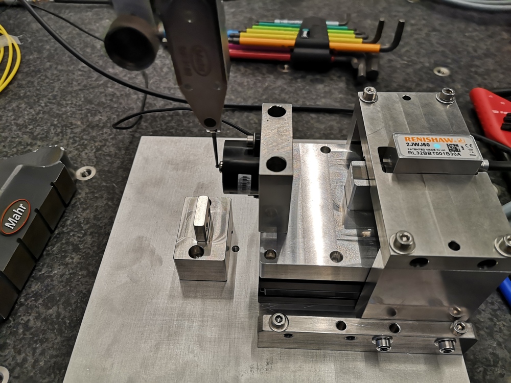
Figure 18: Setup - Top View
Let’s load the measurement results.
load('meas_stiff_probe.mat', 't', 'd', 'dp', 'F')
The time domain measured force and displacement are shown in Figure 19.
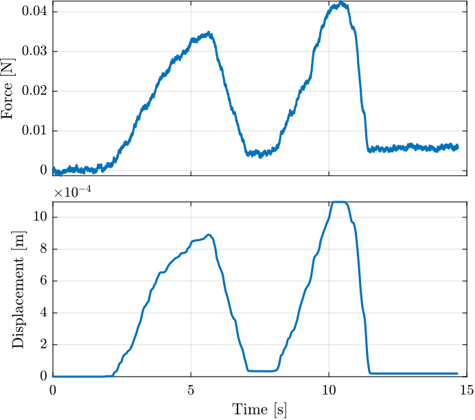
Figure 19: Time domain measurements
Now we can estimate the stiffness with a linear fit.
This is very close to the 0.04 [N/mm] written in the Millimar 1318 probe datasheet.
And compare the linear fit with the raw measurement data (Figure 20).
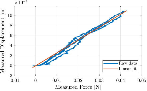
Figure 20: Measured displacement as a function of the measured force. Raw data and linear fit
The Millimar 1318 probe has a stiffness of \(\approx 0.04\,[N/mm]\).
5.3 Force Sensor Calibration
Load Cells:
There are both specified to have \(\pm 1 \%\) of non-linearity over the full range.
The XFL212R has a spherical interface while the FC2231 has a flat surface. Therefore, we should have a nice point contact when using the two force sensors as shown in Figure 21.
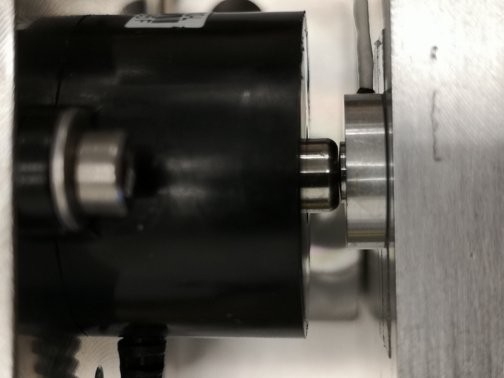
Figure 21: Zoom on the two force sensors in contact
The two force sensors are therefore measuring the exact same force, and we can compare the two measurements.
Let’s load the measured force of both sensors.
%% Load measurement data
load('calibration_force_sensor.mat', 't', 'F', 'Fc')
We remove any offset such that they are both measuring no force when not in contact.
%% Remove offset
F  = F  - mean(F( t > 0.5 & t < 1.0));
Fc = Fc - mean(Fc(t > 0.5 & t < 1.0));
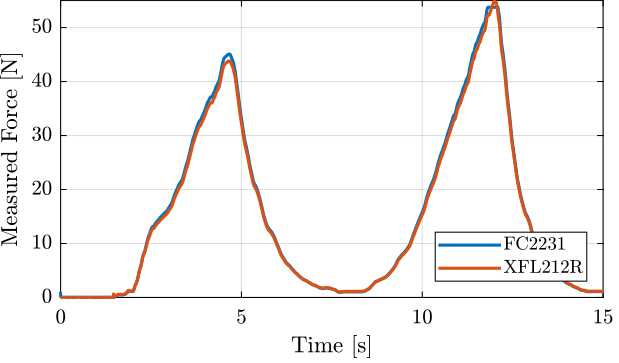
Figure 22: Measured force using both sensors as a function of time
Let’s select only the first part from the moment they are in contact until the maximum force is reached.
%% Only get the first part until maximum force
F  = F( t > 1.55 & t < 4.65);
Fc = Fc(t > 1.55 & t < 4.65);
Then, let’s make a linear fit between the two measured forces.
%% Make a line fit
fit_F = polyfit(Fc, F, 1);
The two forces are plotted against each other as well as the linear fit in Figure 23.
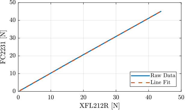
Figure 23: Measured two forces and linear fit
The measurement error between the two sensors is shown in Figure 24. It is below 0.1N for the full measurement range.
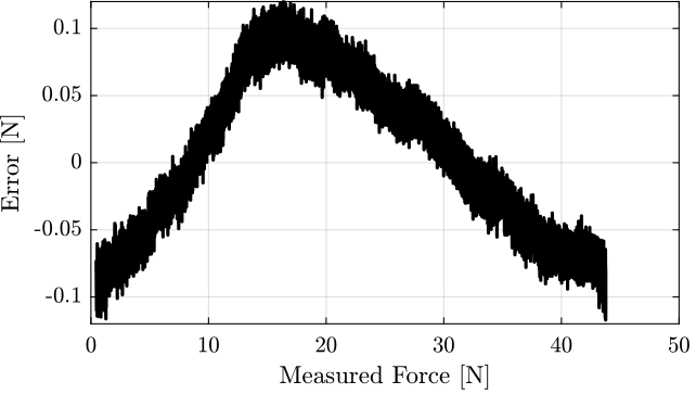
Figure 24: Error in Newtons
The same error is shown in percentage in Figure 25. The error is less than 1% when the measured force is above 5N.
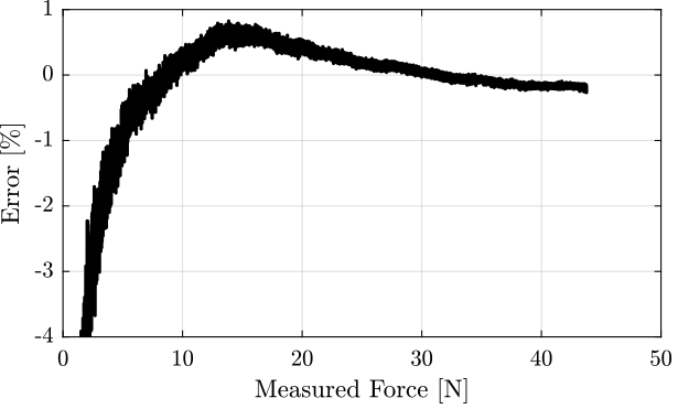
Figure 25: Error in percentage
5.4 Force Sensor Noise
The objective of this measurement is to estimate the noise of the force sensor FC2231-0000-0010-L. To do so, we don’t apply any force to the sensor, and we measure its output for 100s.
Let’s load the measurement data.
%% Load measurement data
load('force_sensor_noise_meas.mat', 't', 'F');
Ts = t(2) - t(1);
The measured force is shown in Figure 26.
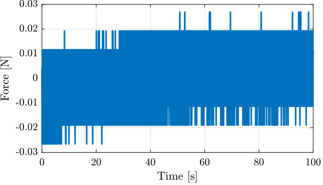
Figure 26: Measured force
Let’s now compute the Amplitude Spectral Density of the measured force.
%% Compute Spectral Density of Measured Force
% Hanning window
win = hanning(ceil(1/Ts));

% Power Spectral Density
[pxx, f] = pwelch(F, win, [], [], 1/Ts);
The results is shown in Figure 27.
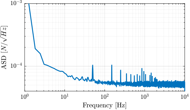
Figure 27: Amplitude Spectral Density of the meaured force
5.5 Force Sensor Stiffness
The objective of this measurement is to estimate the stiffness of the force sensor FC2231-0000-0010-L.
To do so, a very stiff element is fixed in front of the force sensor as shown in Figure 28.
Then, we apply a force on the stiff element through the force sensor. We measure the deflection of the force sensor using an encoder.
Then, having the force and the deflection, we should be able to estimate the stiffness of the force sensor supposing the stiffness of the other elements are much larger.
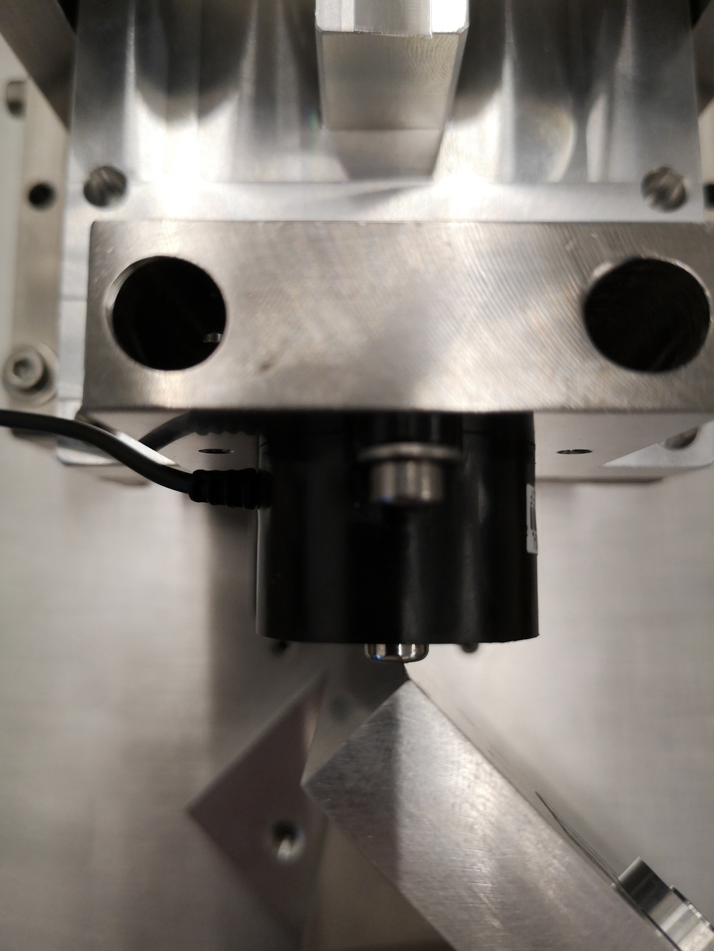
Figure 28: Bench used to measured the stiffness of the force sensor
From the documentation, the deflection of the sensor at the maximum load (50N) is 0.05mm, the stiffness is therefore foreseen to be around \(1\,N/\mu m\).
Let’s load the measured force as well as the measured displacement.
%% Load measurement data
load('force_sensor_stiffness_meas.mat', 't', 'F', 'd')
Some pre-processing is applied on the data.
%% Remove offset
F  = F - mean(F(t > 0.5 & t < 1.0));

%% Select important part of data
F  = F( t > 4.55 & t < 7.24);
d  = d( t > 4.55 & t < 7.24); d = d - d(1);
t  = t( t > 4.55 & t < 7.24);
The linear fit is performed.
%% Linear fit
fit_k = polyfit(F, d, 1);
The displacement as a function of the force as well as the linear fit are shown in Figure 29.
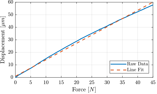
Figure 29: Displacement as a function of the measured force
And we obtain the following stiffness:
k = 0.76 [N/um]
6 Bending Stiffness Measurement
6.1 Introduction
A picture of the bench used to measure the X-bending stiffness of the flexible joints is shown in Figure 30. A closer view on flexible joint is shown in Figure 31 and a zoom on the force sensor tip is shown in Figure 32.
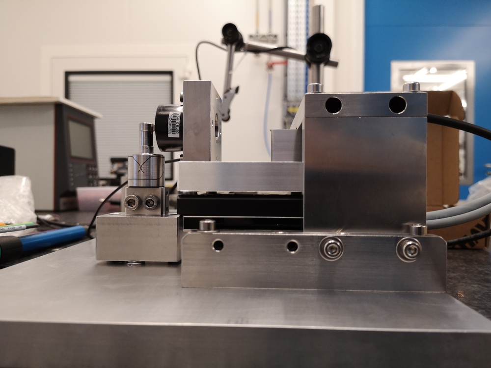
Figure 30: Side view of the flexible joint stiffness bench. X-Bending stiffness is measured.
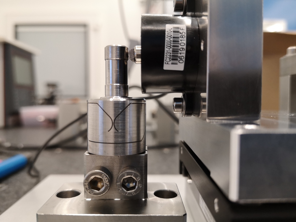
Figure 31: Zoom on the flexible joint - Side view
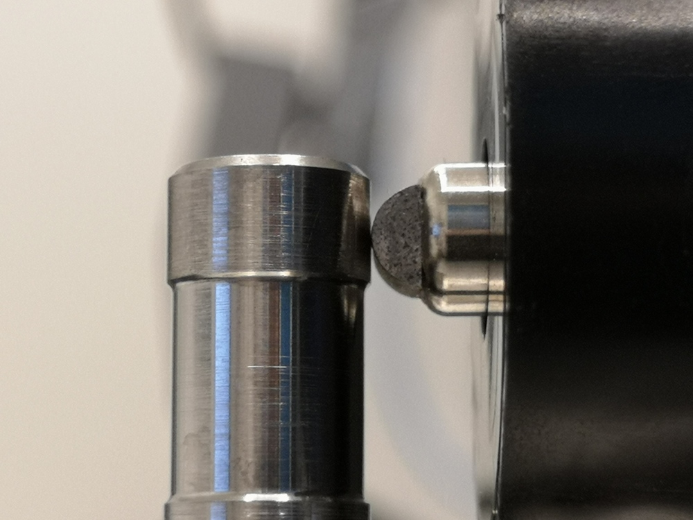
Figure 32: Zoom on the tip of the force sensor
The same bench used to measure the Y-bending stiffness of the flexible joint is shown in Figure 33.
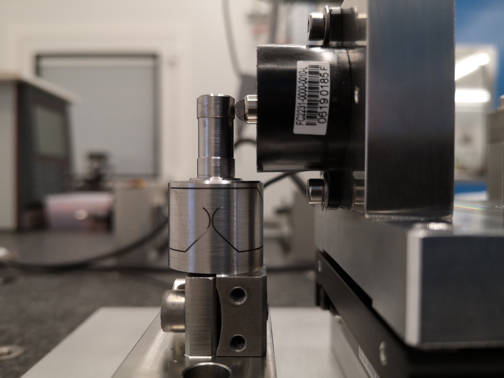
Figure 33: Stiffness measurement bench - Y-d bending measurement
6.2 Analysis of one measurement
In this section is shown how the data are analysis in order to measured:
- the bending stiffness
- the bending stroke
- the stiffness once the mechanical stops are in contact
The height from the flexible joint’s center and the point of application force \(h\) is defined below:
h = 25e-3; % [m]
%% Load Data
load('meas_stiff_flex_1_x.mat', 't', 'F', 'd');

%% Zero the force
F = F - mean(F(t > 0.1 & t < 0.3));

%% Start measurement at t = 0.2 s
d = d(t > 0.2);
F = F(t > 0.2);
t = t(t > 0.2); t = t - t(1);
The obtained time domain measurements are shown in Figure 34.
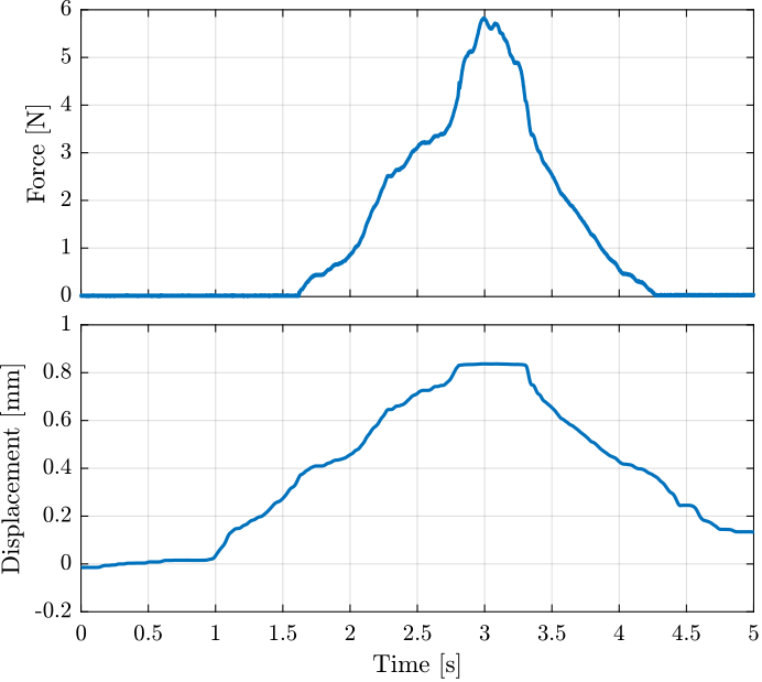
Figure 34: Typical time domain measurements
The displacement as a function of the force is then shown in Figure 35.
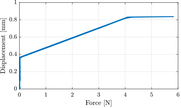
Figure 35: Typical measurement of the diplacement as a function of the applied force
The bending stiffness can be estimated by computing the slope of the curve in Figure 35. The bending stroke and the stiffness when touching the mechanical stop can also be estimated from the same figure.
%% Determine the linear region and region when touching the mechanical stop
% Find when the force sensor touches the flexible joint
i_l_start = find(F > 0.3, 1, 'first');
% Reset the measured diplacement at that point
d = d - d(i_l_start);
% Find then the maximum force is applied
[~, i_s_stop] = max(F);
% Linear region stops ~ when 90% of the stroke is reached
i_l_stop = find(d > 0.9*d(i_s_stop), 1, 'first');
% "Stop" region start ~1N before maximum force is applied
i_s_start = find(F > max(F)-1, 1, 'first');

%% Define variables for the two regions
F_l = F(i_l_start:i_l_stop);
d_l = d(i_l_start:i_l_stop);

F_s = F(i_s_start:i_s_stop);
d_s = d(i_s_start:i_s_stop);
%% Fit the best straight line for the two regions
fit_l = polyfit(F_l, d_l, 1);
fit_s = polyfit(F_s, d_s, 1);

%% Reset displacement based on fit
d = d - fit_l(2);
fit_s(2) = fit_s(2) - fit_l(2);
fit_l(2) = 0;
The raw data as well as the fit corresponding to the two stiffnesses are shown in Figure 36.
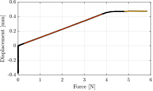
Figure 36: Typical measurement of the diplacement as a function of the applied force with estimated linear fits
Then, the bending stroke is estimated as crossing point between the two fitted lines:
d_max = fit_l(1)*fit_s(2)/(fit_l(1) - fit_s(1));
The obtained characteristics are summarized in Table 5.
| Bending Stiffness [Nm/rad] | 5.5 |
| Bending Stiffness @ stop [Nm/rad] | 173.6 |
| Bending Stroke [mrad] | 18.9 |
6.3 Bending stiffness and bending stroke of all the flexible joints
Now, let’s estimate the bending stiffness and stroke for all the flexible joints.
The results are summarized in Table 6 for the X direction and in Table 7 for the Y direction.
| \(R_{R_x}\) [Nm/rad] | \(k_{R_x,s}\) [Nm/rad] | \(R_{x,\text{max}}\) [mrad] | |
|---|---|---|---|
| 1 | 5.5 | 173.6 | 18.9 |
| 2 | 6.1 | 195.0 | 17.6 |
| 3 | 6.1 | 191.3 | 17.7 |
| 4 | 5.8 | 136.7 | 18.3 |
| 5 | 5.7 | 88.9 | 22.0 |
| 6 | 5.7 | 183.9 | 18.7 |
| 7 | 5.7 | 157.9 | 17.9 |
| 8 | 5.8 | 166.1 | 17.9 |
| 9 | 5.8 | 159.5 | 18.2 |
| 10 | 6.0 | 143.6 | 18.1 |
| 11 | 5.0 | 163.8 | 17.7 |
| 12 | 6.1 | 111.9 | 17.0 |
| 13 | 6.0 | 142.0 | 17.4 |
| 14 | 5.8 | 130.1 | 17.9 |
| 15 | 5.7 | 170.7 | 18.6 |
| 16 | 6.0 | 148.7 | 17.5 |
| \(R_{R_y}\) [Nm/rad] | \(k_{R_y,s}\) [Nm/rad] | \(R_{y,\text{may}}\) [mrad] | |
|---|---|---|---|
| 1 | 5.7 | 323.5 | 17.9 |
| 2 | 5.9 | 306.0 | 17.2 |
| 3 | 6.0 | 224.4 | 16.8 |
| 4 | 5.7 | 247.3 | 17.8 |
| 5 | 5.8 | 250.9 | 13.0 |
| 6 | 5.8 | 244.5 | 17.8 |
| 7 | 5.3 | 214.8 | 18.1 |
| 8 | 5.8 | 217.2 | 17.6 |
| 9 | 5.7 | 225.0 | 17.6 |
| 10 | 6.0 | 254.7 | 17.3 |
| 11 | 4.9 | 261.1 | 18.4 |
| 12 | 5.9 | 161.5 | 16.7 |
| 13 | 6.1 | 227.6 | 16.8 |
| 14 | 5.9 | 221.3 | 17.8 |
| 15 | 5.4 | 241.5 | 17.8 |
| 16 | 5.3 | 291.1 | 17.7 |
6.4 Analysis
The dispersion of the measured bending stiffness is shown in Figure 37 and of the bending stroke in Figure 38.
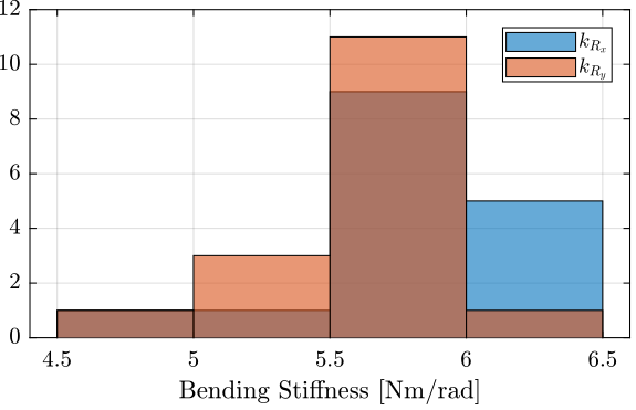
Figure 37: Histogram of the measured bending stiffness
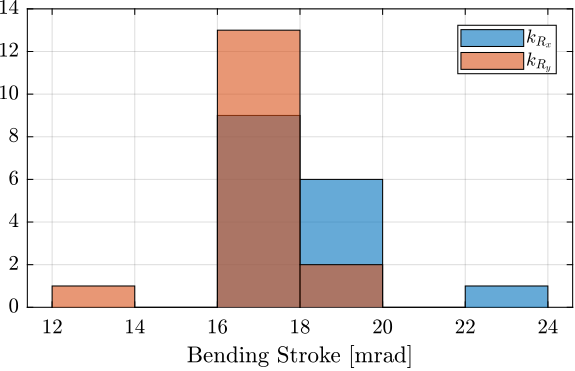
Figure 38: Histogram of the measured bending stroke
The relation between the measured beam thickness and the measured bending stiffness is shown in Figure 39.
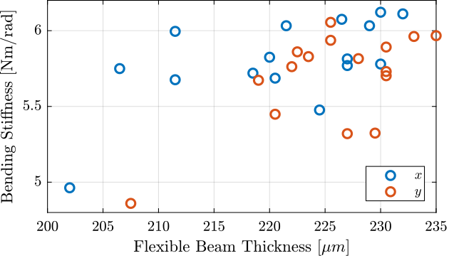
Figure 39: Measured bending stiffness as a function of the estimated flexible beam thickness
6.5 Conclusion
The measured bending stiffness and bending stroke of the flexible joints are very close to the estimated one using a Finite Element Model.
The characteristics of all the flexible joints are also quite close to each other. This should allow us to model them with unique parameters.