Piezoelectric Force Sensor - Test Bench
Table of Contents
- 1. Change of Stiffness due to Sensors stack being open/closed circuit
- 2. Effect of a Resistor in Parallel with the Stack Sensor
- 2.1. Excitation steps and measured generated voltage
- 2.2. Estimation of the voltage offset and discharge time constant
- 2.3. Estimation of the ADC input impedance
- 2.4. Explanation of the Voltage offset
- 2.5. Effect of an additional Parallel Resistor
- 2.6. Obtained voltage offset and time constant with the added resistor
- 3. Generated Number of Charge / Voltage
In this document is studied how a piezoelectric stack can be used to measured the force.
It is divided in the following sections:
- Section 1: the effect of the input impedance of the electronics connected to the force sensor stack on the stiffness of the stack is studied
- Section 2: the effect of a resistor in parallel with the sensor stack is studied
- Section 3: the voltage / number of charge generated by the sensor as a function of the displacement is measured
1 Change of Stiffness due to Sensors stack being open/closed circuit
The experimental Setup is schematically represented in Figure 1.
The dynamics from the voltage \(u\) used to drive the actuator stacks to the encoder displacement \(d_e\) is identified when the switch connected to the sensor stack is either open or closed.
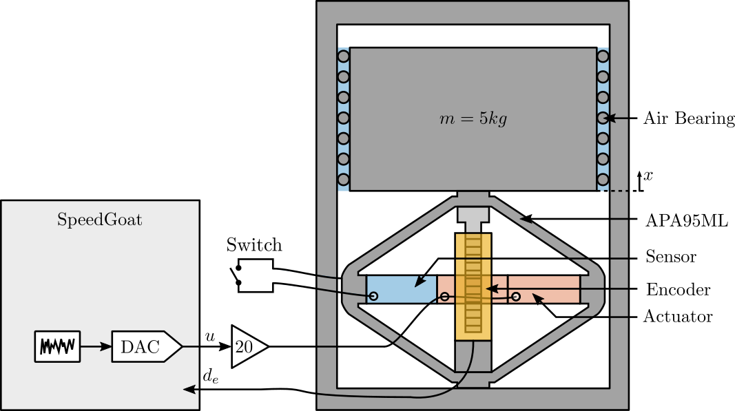
Figure 1: Schematic of the Experiment
When the switch is opened, this correspond of having a measurement electronics with an high input impedance such as a voltage amplifier. When the switch is closed, this correspond of having a measurement electronics with an small input impedance such as a charge amplifier.
We wish here to see how the system dynamics is changing in the two extreme cases.
1.1 Load Data
oc = load('identification_open_circuit.mat', 't', 'encoder', 'u');
sc = load('identification_short_circuit.mat', 't', 'encoder', 'u');
1.2 Transfer Functions
Ts = 1e-4; % Sampling Time [s]
win = hann(ceil(10/Ts));
[tf_oc_est, f] = tfestimate(oc.u, oc.encoder, win, [], [], 1/Ts);
[co_oc_est, ~] = mscohere(  oc.u, oc.encoder, win, [], [], 1/Ts);

[tf_sc_est, ~] = tfestimate(sc.u, sc.encoder, win, [], [], 1/Ts);
[co_sc_est, ~] = mscohere(  sc.u, sc.encoder, win, [], [], 1/Ts);
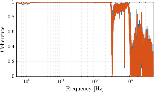
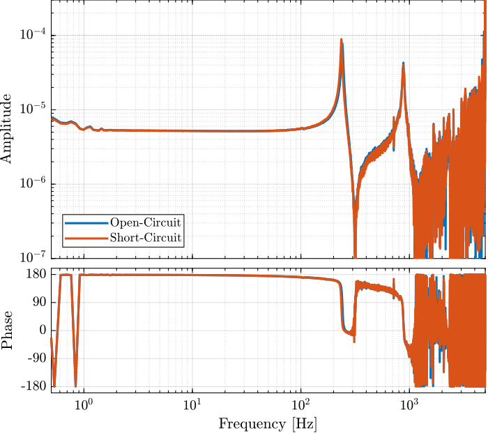
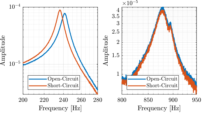
Figure 4: Zoom on the change of resonance
The change of resonance frequency / stiffness is very small and is not important here.
2 Effect of a Resistor in Parallel with the Stack Sensor
The setup is shown in Figure 5 where two stacks are used as actuator (in parallel) and one stack is used as sensor. The voltage amplifier used has a gain of 20 [V/V] (Cedrat LA75B).
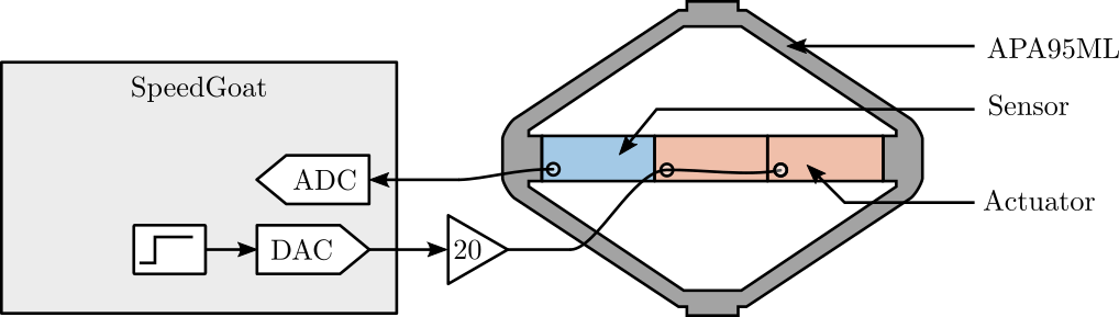
Figure 5: Schematic of the setup
2.1 Excitation steps and measured generated voltage
The measured data is loaded.
load('force_sensor_steps.mat', 't', 'encoder', 'u', 'v');
The excitation signal (steps) and measured voltage across the sensor stack are shown in Figure 6.
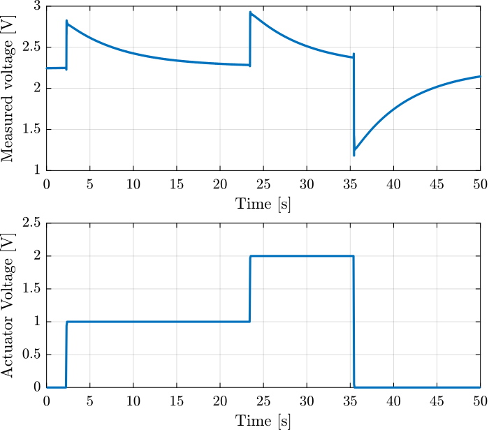
Figure 6: Time domain signal during the 3 actuator voltage steps
2.2 Estimation of the voltage offset and discharge time constant
The measured voltage shows an exponential decay which indicates that the charge across the capacitor formed by the stack is discharging into a resistor. This corresponds to an RC circuit with a time constant \(\tau = RC\).
In order to estimate the time domain, we fit the data with an exponential. The fit function is:
f = @(b,x) b(1).*exp(b(2).*x) + b(3);
Three steps are performed at the following time intervals:
t_s = [ 2.5, 23;
       23.8, 35;
       35.8, 50];
We are interested by the b(2) term, which is the time constant of the exponential.
tau = zeros(size(t_s, 1),1);
V0  = zeros(size(t_s, 1),1);
for t_i = 1:size(t_s, 1)
    t_cur = t(t_s(t_i, 1) < t & t < t_s(t_i, 2));
    t_cur = t_cur - t_cur(1);
    y_cur = v(t_s(t_i, 1) < t & t < t_s(t_i, 2));

    nrmrsd = @(b) norm(y_cur - f(b,t_cur)); % Residual Norm Cost Function
    B0 = [0.5, -0.15, 2.2];                        % Choose Appropriate Initial Estimates
    [B,rnrm] = fminsearch(nrmrsd, B0);     % Estimate Parameters ‘B’

    tau(t_i) = 1/B(2);
    V0(t_i)  = B(3);
end
The obtained values are shown below.
| \(tau\) [s] | \(V_0\) [V] |
|---|---|
| 6.47 | 2.26 |
| 6.76 | 2.26 |
| 6.49 | 2.25 |
2.3 Estimation of the ADC input impedance
With the capacitance being \(C = 4.4 \mu F\), the internal impedance of the Speedgoat ADC can be computed as follows:
Cp = 4.4e-6; % [F]
Rin = abs(mean(tau))/Cp;
1494100.0
The input impedance of the Speedgoat’s ADC should then be close to \(1.5\,M\Omega\) (specified at \(1\,M\Omega\)).
2.4 Explanation of the Voltage offset
As shown in Figure 6, the voltage across the Piezoelectric sensor stack shows a constant voltage offset.
We can explain this offset by looking at the electrical model shown in Figure 7 (taken from (Reza and Andrew 2006)).
The differential amplifier in the Speedgoat has some input bias current \(i_n\) that produces a voltage offset across its own internal resistance. Note that the impedance of the piezoelectric stack is much larger that that at DC.
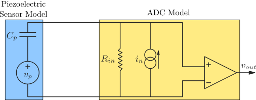
Figure 7: Model of a piezoelectric transducer (left) and instrumentation amplifier (right)
The estimated input bias current is then:
in = mean(V0)/Rin;
1.5119e-06
2.5 Effect of an additional Parallel Resistor
Be looking at Figure 7, we can see that an additional resistor in parallel with \(R_{in}\) would have two effects:
- reduce the input voltage offset \[ V_{off} = \frac{R_a R_{in}}{R_a + R_{in}} i_n \]
- increase the high pass corner frequency \(f_c\) \[ C_p \frac{R_{in}R_a}{R_{in} + R_a} = \tau_c = \frac{1}{f_c} \] \[ R_a = \frac{R_i}{f_c C_p R_i - 1} \]
If we allow the high pass corner frequency to be equals to 3Hz:
fc = 3;
Ra = Rin/(fc*Cp*Rin - 1);
79804
With this parallel resistance value, the voltage offset would be:
V_offset = Ra*Rin/(Ra + Rin) * in;
0.11454
Which is much more acceptable.
A resistor \(R_p \approx 100\,k\Omega\) is then added in parallel with the force sensor as shown in Figure 8.
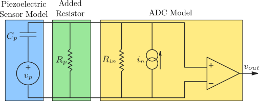
Figure 8: Model of a piezoelectric transducer (left) and instrumentation amplifier (right) with the additional resistor \(R_p\)
2.6 Obtained voltage offset and time constant with the added resistor
After the resistor is added, the same steps response is performed.
load('force_sensor_steps_R_82k7.mat', 't', 'encoder', 'u', 'v');
The results are shown in Figure 9.
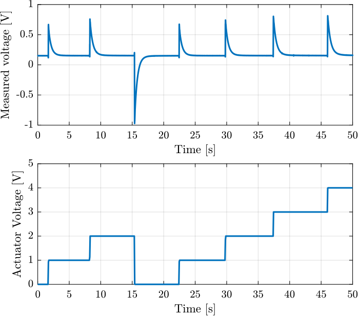
Figure 9: Time domain signal during the actuator voltage steps
Three steps are performed at the following time intervals:
t_s = [1.9,  6;
       8.5, 13;
      15.5, 21;
      22.6, 26;
      30.0, 36;
      37.5, 41;
      46.2, 49.5]
The time constant and voltage offset are again estimated using a fit function. And indeed, we obtain a much smaller offset voltage and a much faster time constant.
| \(tau\) [s] | \(V_0\) [V] |
|---|---|
| 0.43 | 0.15 |
| 0.45 | 0.16 |
| 0.43 | 0.15 |
| 0.43 | 0.15 |
| 0.45 | 0.15 |
| 0.46 | 0.16 |
| 0.48 | 0.16 |
Knowing the capacitance value, we can estimate the value of the added resistor (neglecting the input impedance of \(\approx 1\,M\Omega\)):
Cp = 4.4e-6; % [F]
Rin = abs(mean(tau))/Cp;
101200.0
And we can verify that the bias current estimation stays the same:
in = mean(V0)/Rin;
1.5305e-06
This validates the model of the ADC and the effectiveness of the added resistor.
3 Generated Number of Charge / Voltage
In this section, we wish to estimate the relation between the displacement performed by the stack actuator and the generated voltage/charge on the sensor stack.
3.1 Data Loading
The measured data is loaded and the first 25 seconds of data corresponding to transient data are removed.
load('force_sensor_sin.mat', 't', 'encoder', 'u', 'v');

u       = u(t>25);
v       = v(t>25);
encoder = encoder(t>25) - mean(encoder(t>25));
t       = t(t>25);
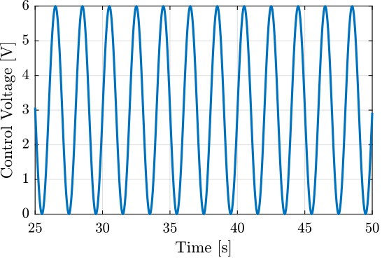
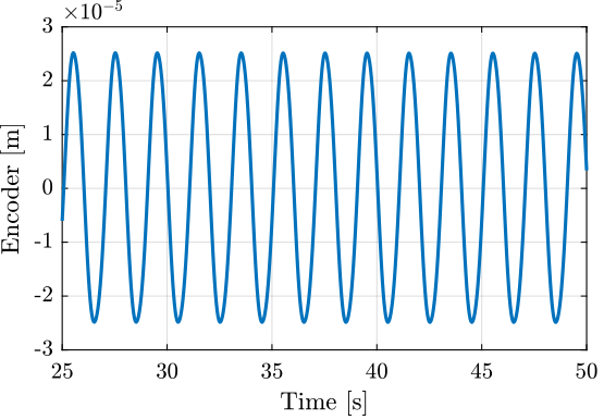
3.2 Excitation signal and corresponding displacement
3.3 Generated Voltage
The generated voltage by the stack is shown in Figure 12.
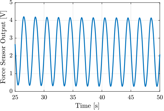
Figure 12: Voltage measured on the stack used as a sensor
3.4 Generated Charge
The capacitance of the stack is
Cp = 4.4e-6; % [F]
The voltage and charge across a capacitor are related through the following equation:
\begin{equation} U_C = \frac{Q}{C} \end{equation}where \(U_C\) is the voltage in Volts, \(Q\) the charge in Coulombs and \(C\) the capacitance in Farads.
The corresponding generated charge is then shown in Figure 13.
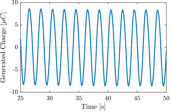
Figure 13: Generated Charge
3.5 Generated Voltage/Charge as a function of the displacement
The relation between the generated voltage and the measured displacement is almost linear as shown in Figure 14.
b1 = encoder\(v-mean(v));
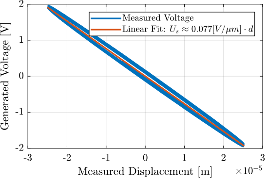
Figure 14: Almost linear relation between the relative displacement and the generated voltage
With a 16bits ADC, the resolution will then be equals to (in [nm]):
abs((20/2^16)/(b1/1e9))
3.9838