Test Bench - Amplified Piezoelectric Actuator
Table of Contents
- 1. Experimental Setup
- 2. Estimation of electrical/mechanical relationships
- 3. Simscape model of the test-bench
- 4. Measurement of the ambient noise in the system
- 5. Identification of the dynamics from actuator Voltage to displacement
- 6. Identification of the dynamics from actuator Voltage to force sensor Voltage
- 7. Integral Force Feedback
This document is divided in the following sections:
- Section 1: the experimental setup is described
- Section 2: the parameters which are important for the Simscape model of the piezoelectric stack actuator and sensors are estimated
- Section 3: the Simscape model of the test bench is presented
- Section 4: as usual, a first measurement of the noise/disturbances present in the system is performed
- Section 5: the transfer function from the actuator voltage to the displacement of the mass is identified and compared with the model
- Section 6: the tranfer function from the actuator voltage to the sensor stack voltage is identified and compare with the model
- Section 7: the Integral Force Feedback control architecture is applied on the system using the force sensor stack in order to add damping to the suspension resonance
1 Experimental Setup
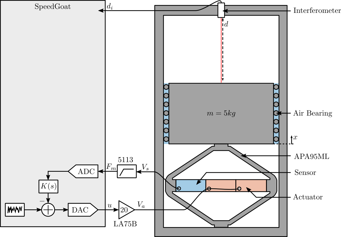
A schematic of the test-bench is shown in Figure 1.
A mass can be vertically moved using the amplified piezoelectric actuator (APA95ML). The displacement of the mass (relative to the mechanical frame) is measured by the interferometer.
The APA95ML has three stacks that can be used as actuator or as sensors.
Pictures of the test bench are shown in Figure 2 and 3.
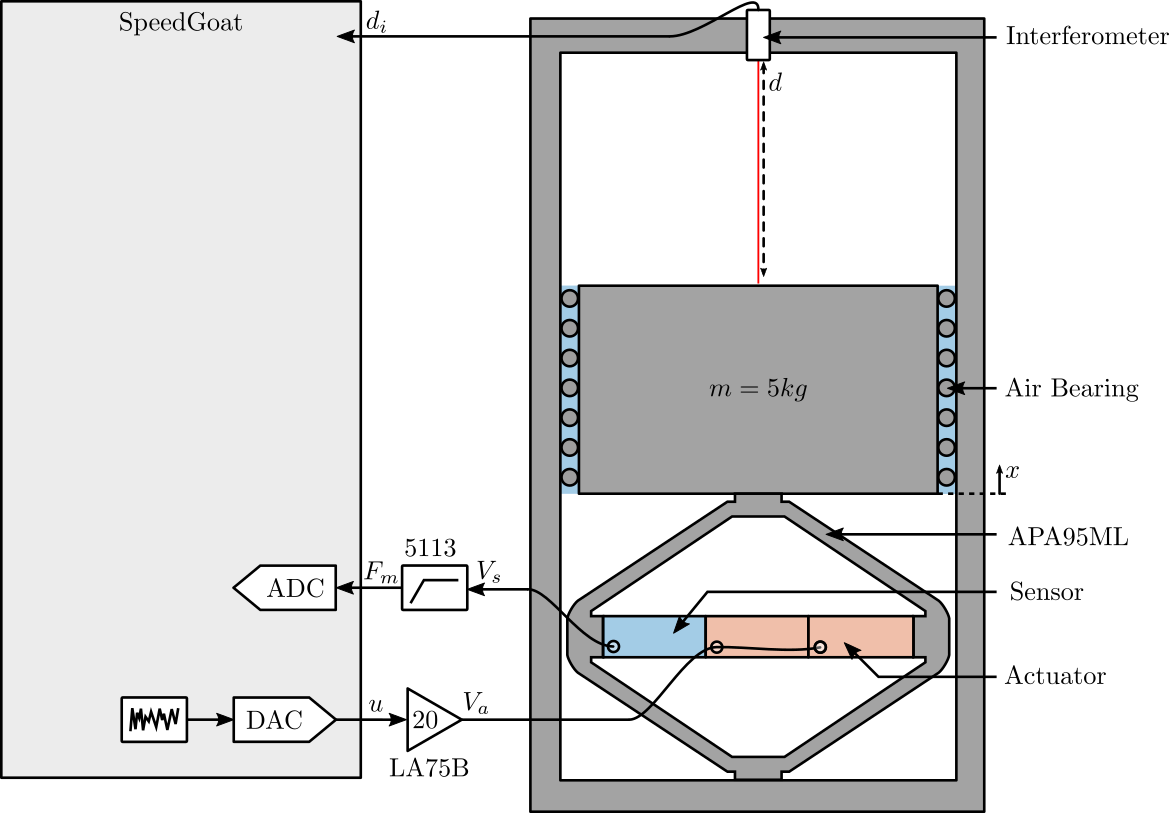
Figure 1: Schematic of the Setup
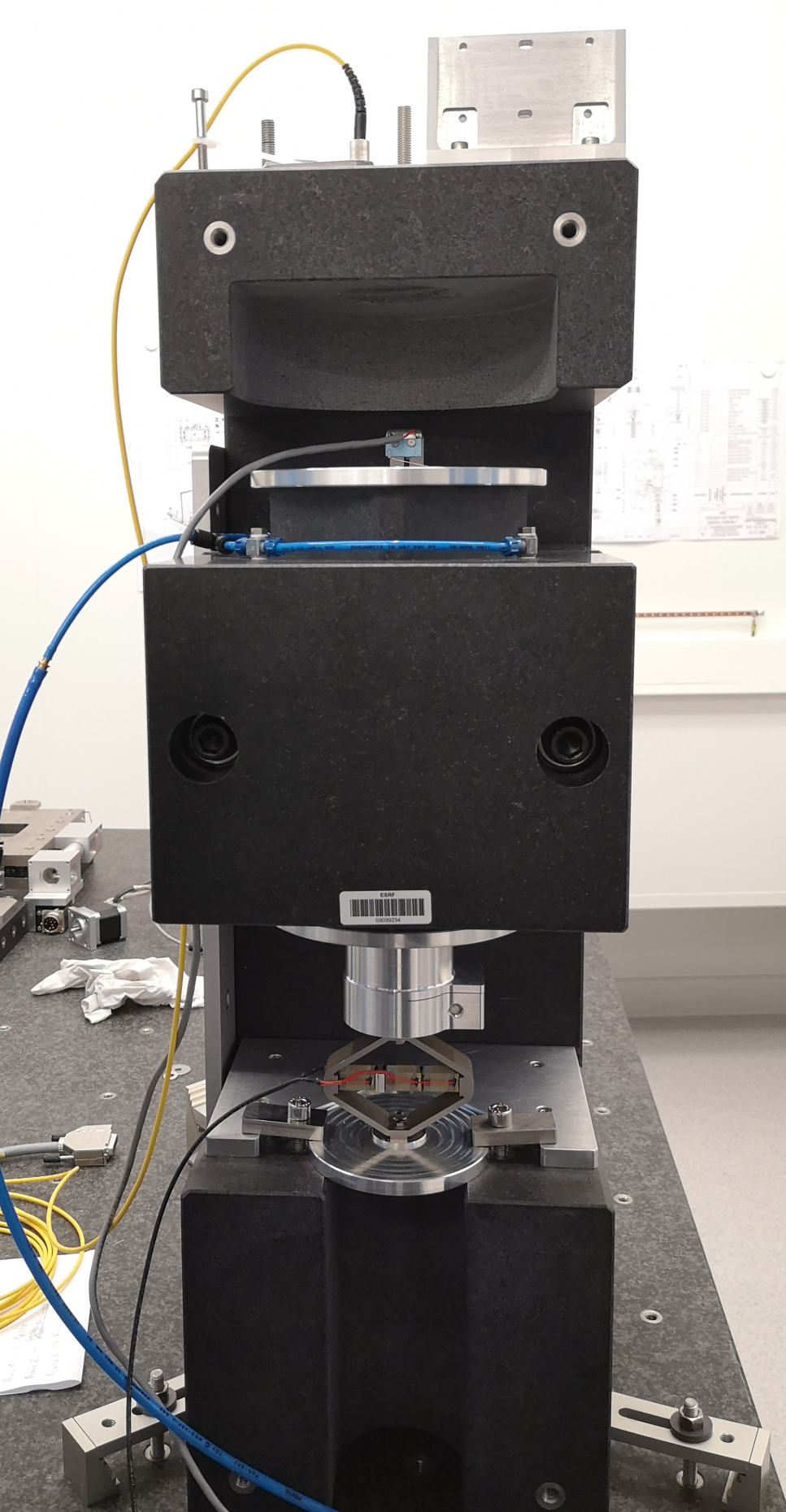
Figure 2: Picture of the Setup
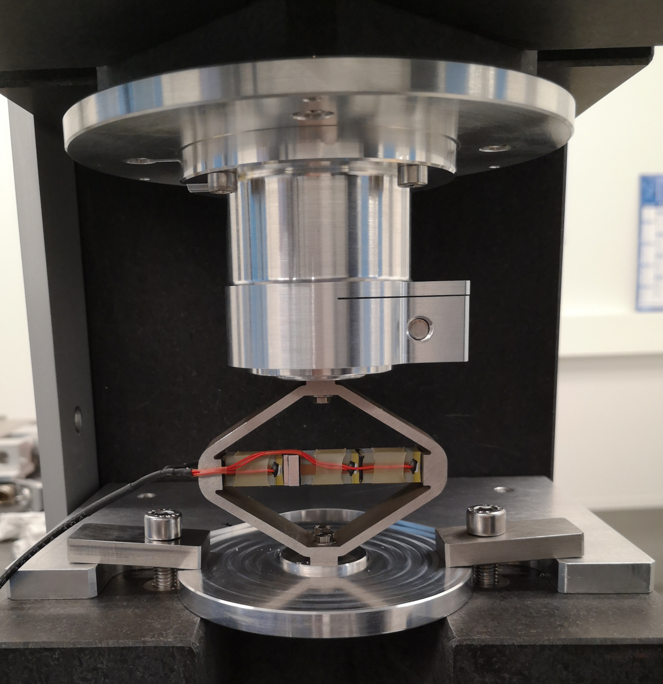
Figure 3: Zoom on the APA
2 Estimation of electrical/mechanical relationships
In order to correctly model the piezoelectric actuator with Simscape, we need to determine:
- \(g_a\): the ratio of the generated force \(F_a\) to the supply voltage \(V_a\) across the piezoelectric stack
- \(g_s\): the ratio of the generated voltage \(V_s\) across the piezoelectric stack when subject to a strain \(\Delta h\)
We estimate \(g_a\) and \(g_s\) using different approaches:
2.1 Estimation from Data-sheet
The stack parameters taken from the data-sheet are shown in Table 1.
| Parameter | Unit | Value |
|---|---|---|
| Nominal Stroke | \(\mu m\) | 20 |
| Blocked force | \(N\) | 4700 |
| Stiffness | \(N/\mu m\) | 235 |
| Voltage Range | \(V\) | -20..150 |
| Capacitance | \(\mu F\) | 4.4 |
| Length | \(mm\) | 20 |
| Stack Area | \(mm^2\) | 10x10 |
Let’s compute the generated force
The stroke is \(L_{\max} = 20\mu m\) for a voltage range of \(V_{\max} = 170 V\). Furthermore, the stiffness is \(k_a = 235 \cdot 10^6 N/m\).
The relation between the applied voltage and the generated force can be estimated as follows:
\begin{equation} g_a = k_a \frac{L_{\max}}{V_{\max}} \end{equation}ka = 235e6; % [N/m] Lmax = 20e-6; % [m] Vmax = 170; % [V]
ga = ka*Lmax/Vmax; % [N/V]
ga = 27.6 [N/V]
From the parameters of the stack, it seems not possible to estimate the relation between the strain and the generated voltage.
2.2 Estimation from Piezoelectric parameters
In order to make the conversion from applied voltage to generated force or from the strain to the generated voltage, we need to defined some parameters corresponding to the piezoelectric material:
d33 = 300e-12; % Strain constant [m/V]
n   = 80;      % Number of layers per stack
ka  = 235e6;   % Stack stiffness [N/m]
The ratio of the developed force to applied voltage is:
\begin{equation} \label{org6f1476c} F_a = g_a V_a, \quad g_a = d_{33} n k_a \end{equation}where:
- \(F_a\): developed force in [N]
- \(n\): number of layers of the actuator stack
- \(d_{33}\): strain constant in [m/V]
- \(k_a\): actuator stack stiffness in [N/m]
- \(V_a\): applied voltage in [V]
If we take the numerical values, we obtain:
ga = d33*n*ka; % [N/V]
ga = 5.6 [N/V]
From (Fleming and Leang 2014) (page 123), the relation between relative displacement of the sensor stack and generated voltage is:
\begin{equation} \label{org43f15ff} V_s = \frac{d_{33}}{\epsilon^T s^D n} \Delta h \end{equation}where:
- \(V_s\): measured voltage in [V]
- \(d_{33}\): strain constant in [m/V]
- \(\epsilon^T\): permittivity under constant stress in [F/m]
- \(s^D\): elastic compliance under constant electric displacement in [m^2/N]
- \(n\): number of layers of the sensor stack
- \(\Delta h\): relative displacement in [m]
If we take the numerical values, we obtain:
d33 = 300e-12; % Strain constant [m/V]
n   = 80;      % Number of layers per stack
eT  = 5.3e-9;  % Permittivity under constant stress [F/m]
sD  = 2e-11;   % Compliance under constant electric displacement [m2/N]
gs = d33/(eT*sD*n); % [V/m]
gs = 35.4 [V/um]
2.3 Estimation from Experiment
The idea here is to obtain the parameters \(g_a\) and \(g_s\) from the comparison of an experimental identification and the identification using Simscape.
Using the experimental identification, we can easily obtain the gain from the applied voltage to the generated displacement, but not to the generated force. However, from the Simscape model, we can easily have the link from the generated force to the displacement, them we can computed \(g_a\).
Similarly, it is fairly easy to experimentally obtain the gain from the stack displacement to the generated voltage across the stack. To link that to the strain of the sensor stack, the simscape model is used.
2.3.1 From actuator voltage \(V_a\) to actuator force \(F_a\)
The data from the identification test is loaded.
load('apa95ml_5kg_Amp_E505.mat', 't', 'um', 'y');

% Any offset value is removed:
um = detrend(um, 0); % Amplifier Input Voltage [V]
y  = detrend(y , 0); % Mass displacement [m]
Now we add a factor 10 to take into account the gain of the voltage amplifier and thus obtain the voltage across the piezoelectric stack.
um = 10*um; % Stack Actuator Input Voltage [V]
Then, the transfer function from the stack voltage to the vertical displacement is computed.
Ts = t(end)/(length(t)-1);
Fs = 1/Ts;

win = hanning(ceil(1*Fs));

[tf_est, f] = tfestimate(um, y, win, [], [], 1/Ts);
The gain from input voltage of the stack to the vertical displacement is determined:
g_d_Va = 4e-7; % [m/V]
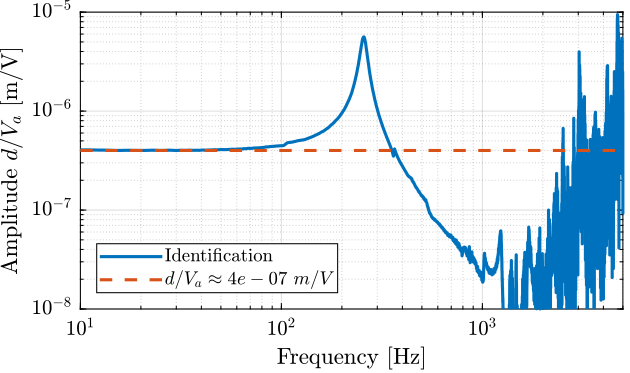
Figure 4: Transfer function from actuator stack voltage \(V_a\) to vertical displacement of the mass \(d\)
Then, the transfer function from forces applied by the stack actuator to the vertical displacement of the mass is identified from the Simscape model.
m = 5.5;

%% Name of the Simulink File
mdl = 'piezo_amplified_3d';

%% Input/Output definition
clear io; io_i = 1;
io(io_i) = linio([mdl, '/Fa'], 1, 'openinput');  io_i = io_i + 1; % Actuator Force [N]
io(io_i) = linio([mdl, '/y'],  1, 'openoutput'); io_i = io_i + 1; % Vertical Displacement [m]

Gd = linearize(mdl, io);
The DC gain the the identified dynamics
g_d_Fa = abs(dcgain(Gd)); % [m/N]
G_d_Fa = 1.2e-08 [m/N]
And finally, the gain \(g_a\) from the the actuator voltage \(V_a\) to the generated force \(F_a\) can be computed:
\begin{equation} g_a = \frac{F_a}{V_a} = \frac{F_a}{d} \frac{d}{V_a} \end{equation}ga = g_d_Va/g_d_Fa;
ga = 33.7 [N/V]
The obtained comparison between the Simscape model and the identified dynamics is shown in Figure 5.
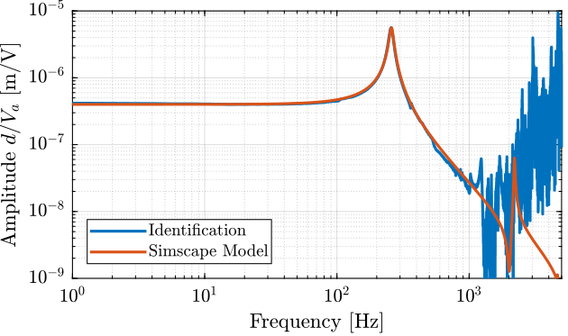
Figure 5: Comparison of the identified transfer function between actuator voltage \(V_a\) and vertical mass displacement \(d\)
2.3.2 From stack strain \(\Delta h\) to generated voltage \(V_s\)
Now, the gain from the stack strain \(\Delta h\) to the generated voltage \(V_s\) is estimated.
We can determine the gain from actuator voltage \(V_a\) to sensor voltage \(V_s\) thanks to the identification. Using the simscape model, we can have the transfer function from the actuator voltage \(V_a\) (using the previously estimated gain \(g_a\)) to the sensor stack strain \(\Delta h\).
Finally, using these two values, we can compute the gain \(g_s\) from the stack strain \(\Delta h\) to the generated Voltage \(V_s\).
Identification data is loaded.
load('apa95ml_5kg_2a_1s.mat', 't', 'u', 'v');

u = detrend(u, 0); % Input Voltage of the Amplifier [V]
v = detrend(v, 0); % Voltage accross the stack sensor [V]
Here, an amplifier with a gain of 20 is used.
u = 20*u; % Input Voltage of the Amplifier [V]
Then, the transfer function from \(V_a\) to \(V_s\) is identified and its DC gain is estimated (Figure 6).
Ts = t(end)/(length(t)-1);
Fs = 1/Ts;

win = hann(ceil(10/Ts));

[tf_est, f] = tfestimate(u, v, win, [], [], 1/Ts);
g_Vs_Va = 0.022; % [V/V]
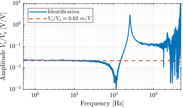
Figure 6: Transfer function from actuator stack voltage \(V_a\) to sensor stack voltage \(V_s\)
Now the transfer function from the actuator stack voltage to the sensor stack strain is estimated using the Simscape model.
m = 5.5;

%% Name of the Simulink File
mdl = 'piezo_amplified_3d';

%% Input/Output definition
clear io; io_i = 1;
io(io_i) = linio([mdl, '/Va'], 1, 'openinput');  io_i = io_i + 1; % Actuator Voltage [V]
io(io_i) = linio([mdl, '/dL'], 1, 'openoutput'); io_i = io_i + 1; % Sensor Stack displacement [m]

Gf = linearize(mdl, io);
The gain from the actuator stack voltage to the sensor stack strain is estimated below.
G_dh_Va = abs(dcgain(Gf));
G_dh_Va = 6.2e-09 [m/V]
And finally, the gain \(g_s\) from the sensor stack strain to the generated voltage can be estimated:
\begin{equation} g_s = \frac{V_s}{\Delta h} = \frac{V_s}{V_a} \frac{V_a}{\Delta h} \end{equation}gs = g_Vs_Va/G_dh_Va; % [V/m]
gs = 3.5 [V/um]
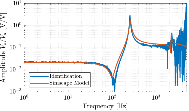
Figure 7: Comparison of the identified transfer function between actuator voltage \(V_a\) and sensor stack voltage
2.4 Conclusion
The obtained parameters \(g_a\) and \(g_s\) are not consistent between the different methods.
The one using the experimental data are saved and further used.
save('./matlab/mat/apa95ml_params.mat', 'ga', 'gs');
3 Simscape model of the test-bench
The idea here is to model the test-bench using Simscape.
Whereas the suspended mass and metrology frame can be considered as rigid bodies in the frequency range of interest, the Amplified Piezoelectric Actuator (APA) is flexible.
To model the APA, a Finite Element Model (FEM) is used (Figure 8) and imported into Simscape.
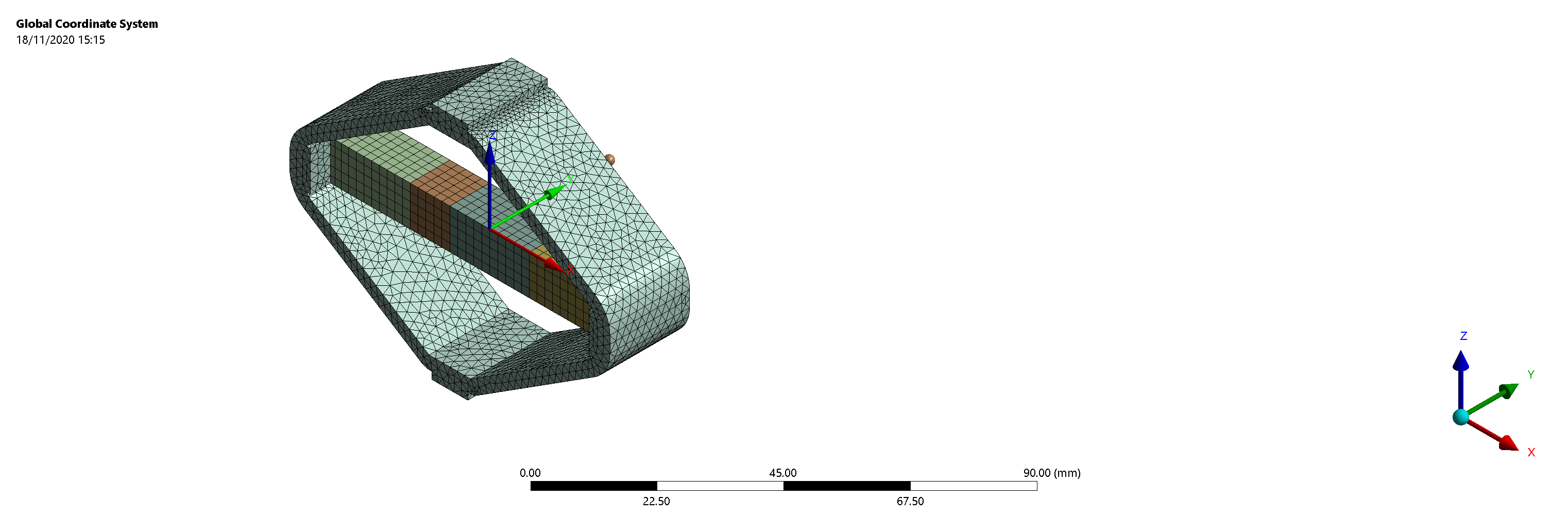
Figure 8: Finite Element Model of the APA95ML
3.1 Import Mass Matrix, Stiffness Matrix, and Interface Nodes Coordinates
We first extract the stiffness and mass matrices.
K = readmatrix('APA95ML_K.CSV');
M = readmatrix('APA95ML_M.CSV');
| 300000000.0 | -1000.0 | -30000.0 | -40.0 | 70000.0 | 300.0 | 20000000.0 | -30.0 | -5000.0 | 5 |
| -1000.0 | 50000000.0 | -7000.0 | 800000.0 | -20.0 | 300.0 | 3000.0 | 5000000.0 | 400.0 | -40000.0 |
| -30000.0 | -7000.0 | 100000000.0 | -200.0 | -60.0 | 70.0 | 3000.0 | 3000.0 | -8000000.0 | -30.0 |
| -40.0 | 800000.0 | -200.0 | 20000.0 | -0.4 | 4 | 30.0 | 40000.0 | 7 | -300.0 |
| 70000.0 | -20.0 | -60.0 | -0.4 | 3000.0 | 1 | -6000.0 | 10.0 | 8 | -0.1 |
| 300.0 | 300.0 | 70.0 | 4 | 1 | 40000.0 | -10.0 | -10.0 | 30.0 | 0.1 |
| 20000000.0 | 3000.0 | 3000.0 | 30.0 | -6000.0 | -10.0 | 300000000.0 | 2000.0 | 9000.0 | -100.0 |
| -30.0 | 5000000.0 | 3000.0 | 40000.0 | 10.0 | -10.0 | 2000.0 | 50000000.0 | -3000.0 | -800000.0 |
| -5000.0 | 400.0 | -8000000.0 | 7 | 8 | 30.0 | 9000.0 | -3000.0 | 100000000.0 | 100.0 |
| 5 | -40000.0 | -30.0 | -300.0 | -0.1 | 0.1 | -100.0 | -800000.0 | 100.0 | 20000.0 |
| 0.03 | 7e-08 | 2e-06 | -3e-09 | -0.0002 | -6e-08 | -0.001 | 8e-07 | 6e-07 | -8e-09 |
| 7e-08 | 0.02 | -1e-06 | 9e-05 | -3e-09 | -4e-09 | -1e-06 | -0.0006 | -4e-08 | 5e-06 |
| 2e-06 | -1e-06 | 0.02 | -3e-08 | -4e-08 | 1e-08 | 1e-07 | -2e-07 | 0.0003 | 1e-09 |
| -3e-09 | 9e-05 | -3e-08 | 1e-06 | -3e-11 | -3e-13 | -7e-09 | -5e-06 | -3e-10 | 3e-08 |
| -0.0002 | -3e-09 | -4e-08 | -3e-11 | 2e-06 | 6e-10 | 2e-06 | -7e-09 | -2e-09 | 7e-11 |
| -6e-08 | -4e-09 | 1e-08 | -3e-13 | 6e-10 | 1e-06 | 1e-08 | 3e-09 | -2e-09 | 2e-13 |
| -0.001 | -1e-06 | 1e-07 | -7e-09 | 2e-06 | 1e-08 | 0.03 | 4e-08 | -2e-06 | 8e-09 |
| 8e-07 | -0.0006 | -2e-07 | -5e-06 | -7e-09 | 3e-09 | 4e-08 | 0.02 | -9e-07 | -9e-05 |
| 6e-07 | -4e-08 | 0.0003 | -3e-10 | -2e-09 | -2e-09 | -2e-06 | -9e-07 | 0.02 | 2e-08 |
| -8e-09 | 5e-06 | 1e-09 | 3e-08 | 7e-11 | 2e-13 | 8e-09 | -9e-05 | 2e-08 | 1e-06 |
Then, we extract the coordinates of the interface nodes.
[int_xyz, int_i, n_xyz, n_i, nodes] = extractNodes('APA95ML_out_nodes_3D.txt');
The interface nodes are shown in Figure 9 and their coordinates are listed in Table 4.
| Total number of Nodes | 7 |
| Number of interface Nodes | 7 |
| Number of Modes | 6 |
| Size of M and K matrices | 48 |
| Node i | Node Number | x [m] | y [m] | z [m] |
|---|---|---|---|---|
| 1.0 | 40467.0 | 0.0 | 0.0 | 0.029997 |
| 2.0 | 40469.0 | 0.0 | 0.0 | -0.029997 |
| 3.0 | 40470.0 | -0.035 | 0.0 | 0.0 |
| 4.0 | 40475.0 | -0.015 | 0.0 | 0.0 |
| 5.0 | 40476.0 | -0.005 | 0.0 | 0.0 |
| 6.0 | 40477.0 | 0.015 | 0.0 | 0.0 |
| 7.0 | 40478.0 | 0.035 | 0.0 | 0.0 |
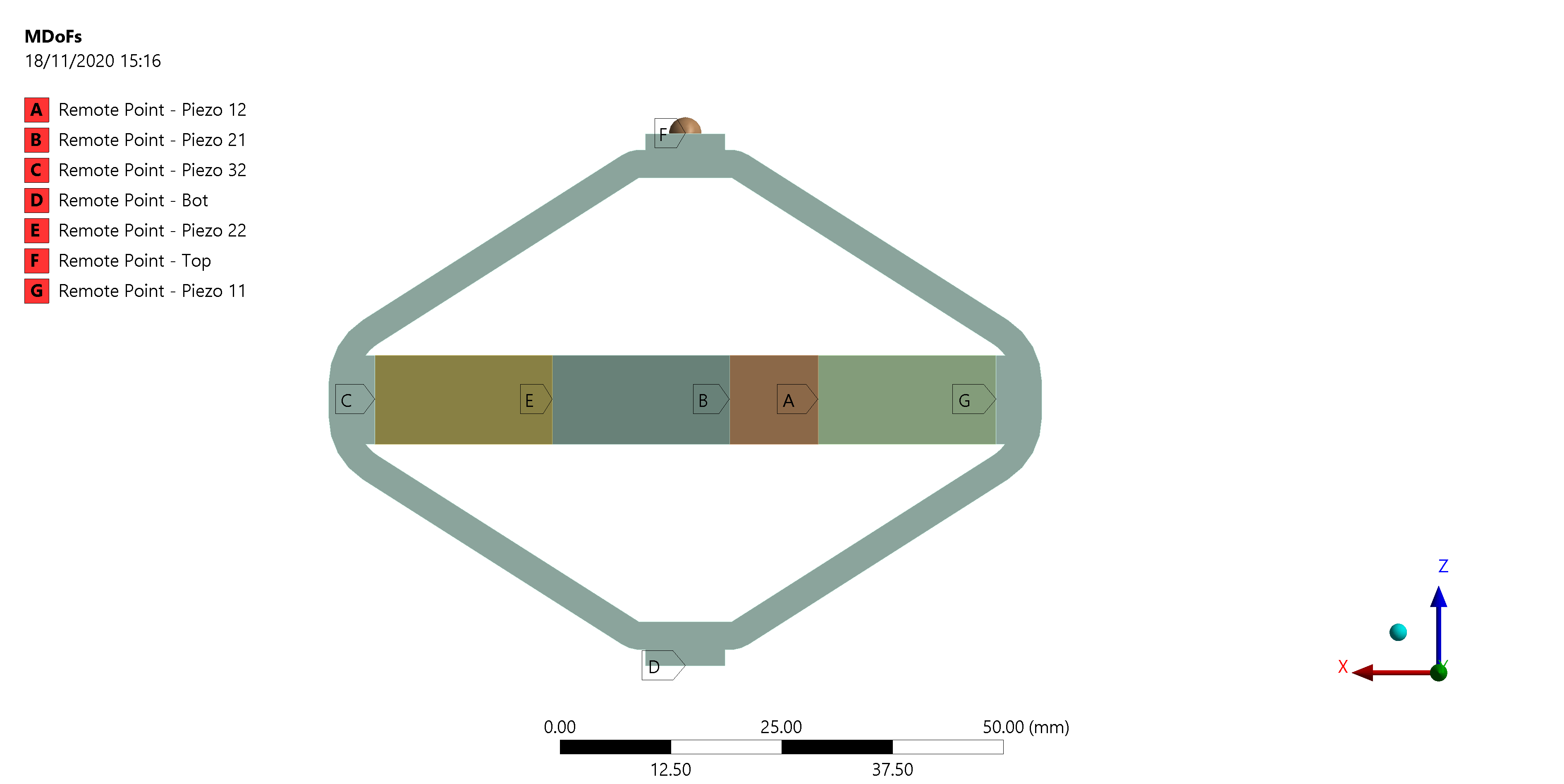
Figure 9: Interface Nodes chosen for the APA95ML
Using K, M and int_xyz, we can use the Reduced Order Flexible Solid simscape block.
3.2 Simscape Model
The flexible element is imported using the Reduced Order Flexible Solid Simscape block.
To model the actuator, an Internal Force block is added between the nodes 3 and 12.
A Relative Motion Sensor block is added between the nodes 1 and 2 to measure the displacement and the amplified piezo.
One mass is fixed at one end of the piezo-electric stack actuator, the other end is fixed to the world frame.
m = 5.5;
load('apa95ml_params.mat', 'ga', 'gs');
3.3 Dynamics from Actuator Voltage to Vertical Mass Displacement
The identified dynamics is shown in Figure 10.
%% Name of the Simulink File
mdl = 'piezo_amplified_3d';

%% Input/Output definition
clear io; io_i = 1;
io(io_i) = linio([mdl, '/Va'], 1, 'openinput');  io_i = io_i + 1; % Actuator Voltage [V]
io(io_i) = linio([mdl, '/y'],  1, 'openoutput'); io_i = io_i + 1; % Vertical Displacement [m]

Ghm = linearize(mdl, io);
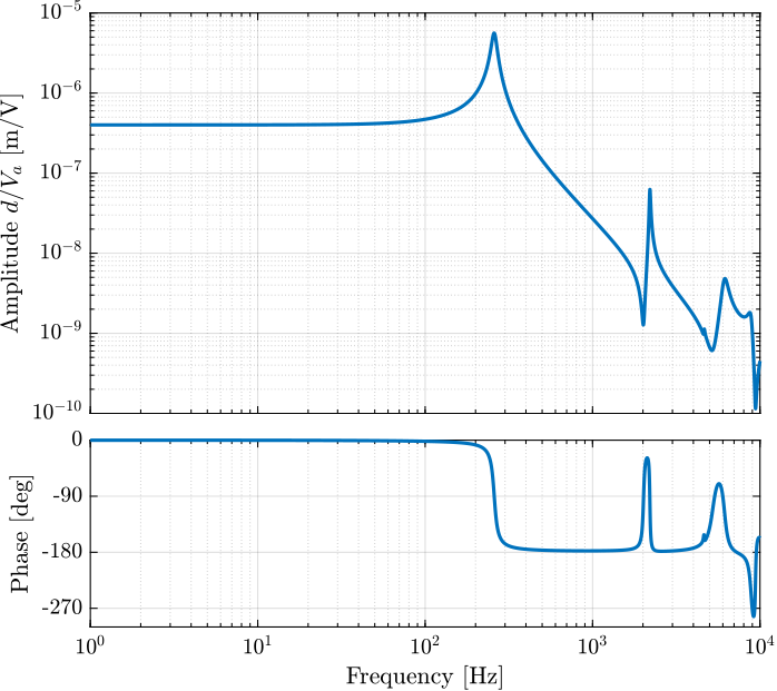
Figure 10: Dynamics from \(F\) to \(d\) without a payload and with a 5kg payload
3.4 Dynamics from Actuator Voltage to Force Sensor Voltage
The obtained dynamics is shown in Figure 11.
%% Name of the Simulink File
mdl = 'piezo_amplified_3d';

%% Input/Output definition
clear io; io_i = 1;
io(io_i) = linio([mdl, '/Va'], 1, 'openinput');  io_i = io_i + 1; % Voltage Actuator [V]
io(io_i) = linio([mdl, '/Vs'], 1, 'openoutput'); io_i = io_i + 1; % Sensor Voltage [V]

Gfm = linearize(mdl, io);
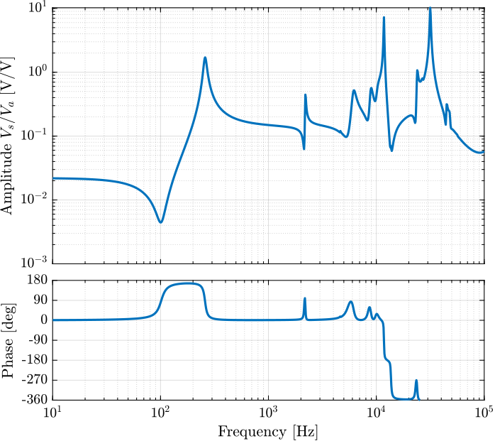
Figure 11: Dynamics from \(F\) to \(F_m\) for \(m=0\) and \(m = 10kg\)
3.5 Save Data for further use
save('matlab/mat/fem_simscape_models.mat', 'Ghm', 'Gfm')
4 Measurement of the ambient noise in the system
This first measurement consist of measuring the displacement of the mass using the interferometer when no voltage is applied to the actuator.
This can help determining the actuator voltage necessary to generate a motion way above the measured noise and disturbances, and thus obtain a good identification.
4.1 Time Domain Data
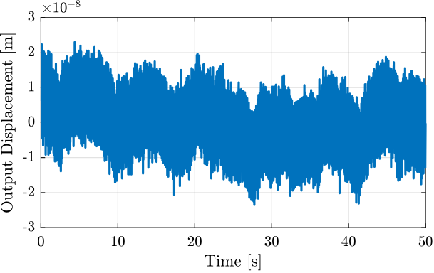
Figure 12: Measurement of the Mass displacement during Huddle Test
4.2 PSD of Measurement Noise
Ts = t(end)/(length(t)-1);
Fs = 1/Ts;

win = hanning(ceil(1*Fs));
[pxx, f] = pwelch(y(1000:end), win, [], [], Fs);
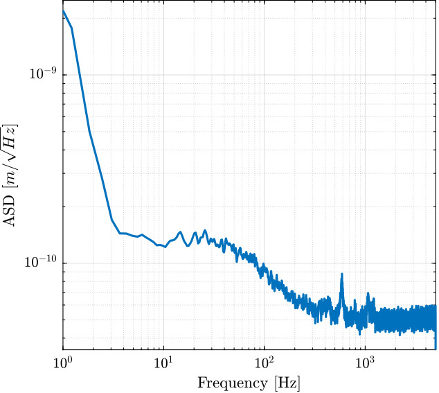
Figure 13: Amplitude Spectral Density of the Displacement during Huddle Test
5 Identification of the dynamics from actuator Voltage to displacement
The setup used for the identification of the dynamics from \(V_a\) to \(d\) is shown in Figure 14.
A Voltage amplifier with a gain of \(10\) is used. Two stacks are used as actuators while one stack is used as a force sensor.
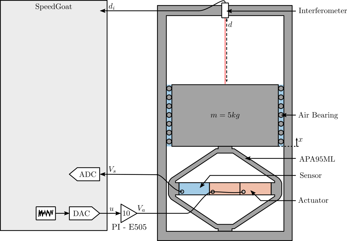
Figure 14: Test Bench used for the identification of the dynaimcs from \(V_a\) to \(d\)
5.1 Load Data
The data from the “noise test” and the identification test are loaded.
ht = load('huddle_test.mat', 't', 'u', 'y');
load('apa95ml_5kg_Amp_E505.mat', 't', 'um', 'y');
Any offset value is removed:
um = detrend(um, 0); % Input Voltage [V]
y  = detrend(y , 0); % Mass displacement [m]

ht.u  = detrend(ht.u, 0);
ht.y  = detrend(ht.y, 0);
Now we add a factor 10 to take into account the gain of the voltage amplifier.
um = 10*um;
5.2 Comparison of the PSD with Huddle Test
Ts = t(end)/(length(t)-1);
Fs = 1/Ts;

win = hanning(ceil(1*Fs));
[pxx, f] = pwelch(y, win, [], [], Fs);
[pht, ~] = pwelch(ht.y, win, [], [], Fs);
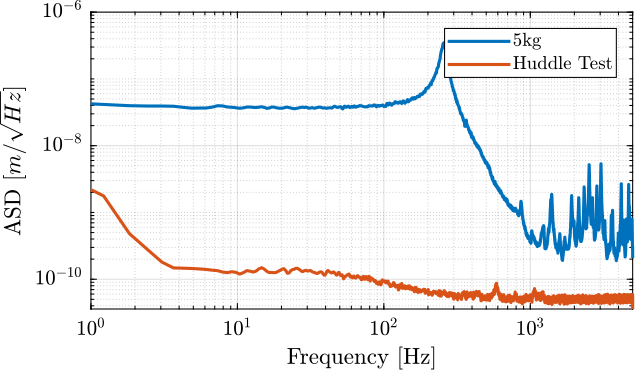
Figure 15: Comparison of the ASD for the identification test and the huddle test
5.3 Compute TF estimate and Coherence
[tf_est, f] = tfestimate(um, -y, win, [], [], 1/Ts);
[co_est, ~] = mscohere(  um, -y, win, [], [], 1/Ts);
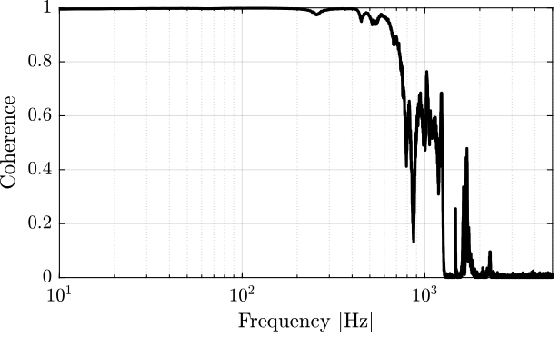
Figure 16: Coherence
Comparison with the FEM model
load('mat/fem_simscape_models.mat', 'Ghm');
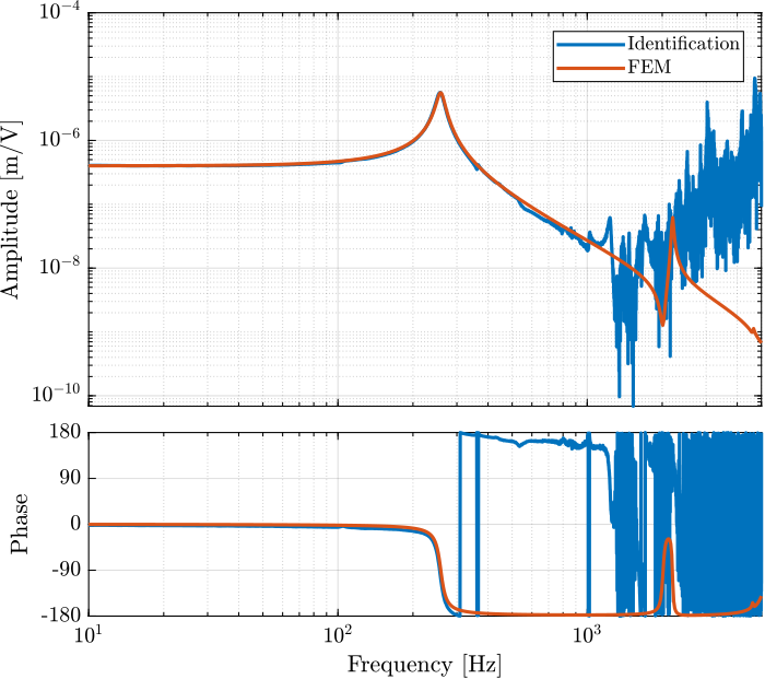
Figure 17: Comparison of the identified transfer function and the one estimated from the FE model
6 Identification of the dynamics from actuator Voltage to force sensor Voltage
The same setup shown in Figure 14 is used.
The data are loaded:
load('apa95ml_5kg_2a_1s.mat', 't', 'u', 'v');
Any offset is removed.
u = detrend(u, 0); % Speedgoat DAC output Voltage [V]
v = detrend(v, 0); % Speedgoat ADC input Voltage (sensor stack) [V]
Here, the amplifier gain is 20.
u = 20*u; % Actuator Stack Voltage [V]
The transfer function from the actuator voltage \(V_a\) to the force sensor stack voltage \(V_s\) is computed.
Ts = t(end)/(length(t)-1);
Fs = 1/Ts;

win = hann(ceil(5/Ts));

[tf_est,  f] = tfestimate(u, v, win, [], [], 1/Ts);
[coh,     ~] = mscohere(  u, v, win, [], [], 1/Ts);
The coherence is shown in Figure 18.
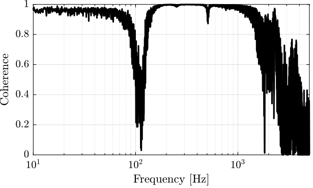
Figure 18: Coherence
The Simscape model is loaded and compared with the identified dynamics in Figure 19. The non-minimum phase zero is just a side effect of the not so great identification. Taking longer measurements would results in a minimum phase zero.
load('mat/fem_simscape_models.mat', 'Gfm');
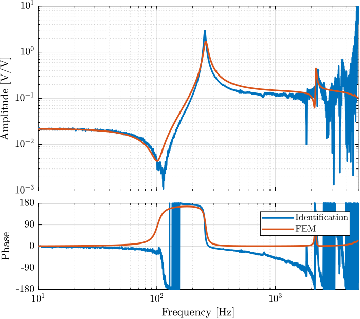
Figure 19: Comparison of the identified dynamics from voltage output to voltage input and the FEM
7 Integral Force Feedback
7.1 IFF Plant
From the identified plant, a model of the transfer function from the actuator stack voltage to the force sensor generated voltage is developed.
w_z = 2*pi*111; % Zeros frequency [rad/s]
w_p = 2*pi*255; % Pole frequency [rad/s]
xi_z = 0.05;
xi_p = 0.015;
G_inf = 0.1;

Gi = G_inf*(s^2 + 2*xi_z*w_z*s + w_z^2)/(s^2 + 2*xi_p*w_p*s + w_p^2);
Its bode plot is shown in Figure 21.
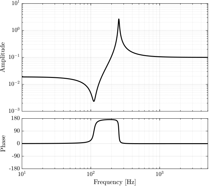
Figure 21: Bode plot of the IFF plant
The controller used in the Integral Force Feedback Architecture is:
\begin{equation} K_{\text{IFF}}(s) = \frac{g}{s + 2\cdot 2\pi} \cdot \frac{s}{s + 0.5 \cdot 2\pi} \end{equation}where \(g\) is a gain that can be tuned.
Above 2 Hz the controller is basically an integrator, whereas an high pass filter is added at 0.5Hz to further reduce the low frequency gain.
In the frequency band of interest, this controller should mostly act as a pure integrator.
The Root Locus corresponding to this controller is shown in Figure 22.
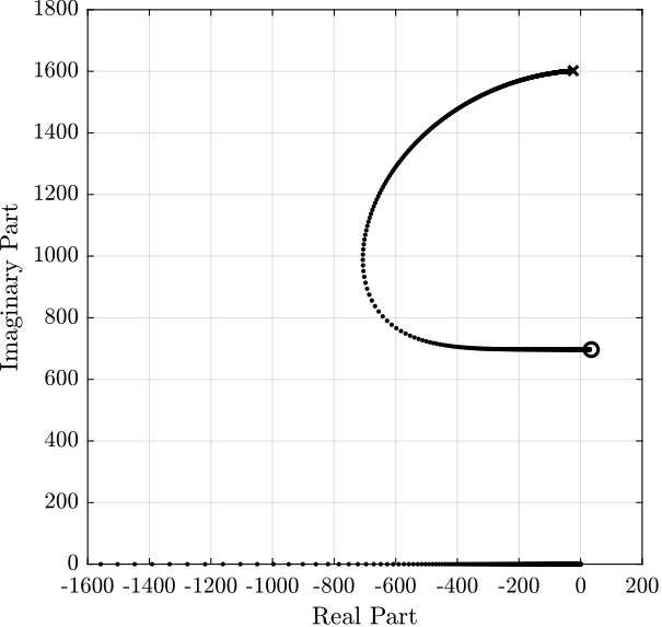
Figure 22: Root Locus for IFF
7.2 First tests with few gains
The controller is now implemented in practice, and few controller gains are tested: \(g = 0\), \(g = 10\) and \(g = 100\).
For each controller gain, the identification shown in Figure 20 is performed.
iff_g10  = load('apa95ml_iff_g10_res.mat',  'u', 't', 'y', 'v');
iff_g100 = load('apa95ml_iff_g100_res.mat', 'u', 't', 'y', 'v');
iff_of   = load('apa95ml_iff_off_res.mat',  'u', 't', 'y', 'v');
Ts = 1e-4;
win = hann(ceil(10/Ts));

[tf_iff_g10, f] = tfestimate(iff_g10.u, iff_g10.y, win, [], [], 1/Ts);
[co_iff_g10, ~] = mscohere(iff_g10.u, iff_g10.y, win, [], [], 1/Ts);

[tf_iff_g100, ~] = tfestimate(iff_g100.u, iff_g100.y, win, [], [], 1/Ts);
[co_iff_g100, ~] = mscohere(iff_g100.u, iff_g100.y, win, [], [], 1/Ts);

[tf_iff_of, ~] = tfestimate(iff_of.u, iff_of.y, win, [], [], 1/Ts);
[co_iff_of, ~] = mscohere(iff_of.u, iff_of.y, win, [], [], 1/Ts);
The coherence between the excitation signal and the mass displacement as measured by the interferometer is shown in Figure 23.
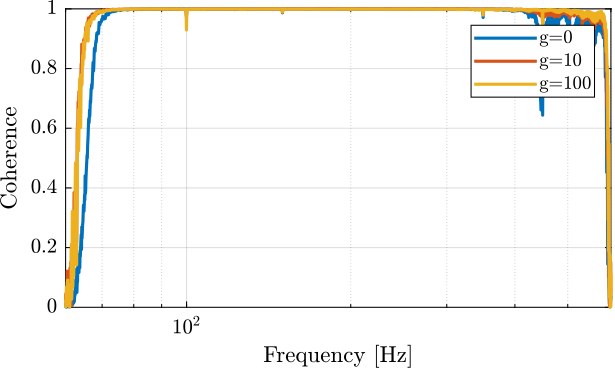
Figure 23: Coherence
The obtained transfer functions are shown in Figure 24. It is clear that the IFF architecture can actively damp the main resonance of the system.
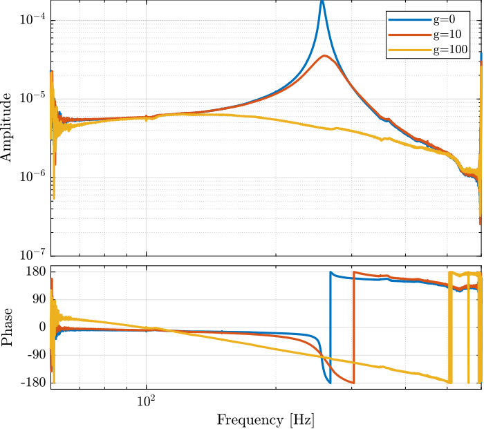
Figure 24: Bode plot for different values of IFF gain
7.3 Second test with many Gains
Then, the same identification test is performed for many more gains.
load('apa95ml_iff_test.mat', 'results');
Ts = 1e-4;
win = hann(ceil(10/Ts));
tf_iff = {zeros(1, length(results))};
co_iff = {zeros(1, length(results))};
g_iff = [0, 1, 5, 10, 50, 100];

for i=1:length(results)
    [tf_est, f] = tfestimate(results{i}.u, results{i}.y, win, [], [], 1/Ts);
    [co_est, ~] = mscohere(results{i}.u, results{i}.y, win, [], [], 1/Ts);

    tf_iff(i) = {tf_est};
    co_iff(i) = {co_est};
end
The obtained dynamics are shown in Figure 25.
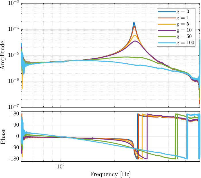
Figure 25: Identified dynamics from excitation voltage to the mass displacement
For each gain, the parameters of a second order resonant system that best fits the data are estimated and are compared with the data in Figure 26.
G_id = {zeros(1,length(results))};

f_start = 70; % [Hz]
f_end = 500; % [Hz]

for i = 1:length(results)
    tf_id = tf_iff{i}(sum(f<f_start):length(f)-sum(f>f_end));
    f_id = f(sum(f<f_start):length(f)-sum(f>f_end));

    gfr = idfrd(tf_id, 2*pi*f_id, Ts);
    G_id(i) = {procest(gfr,'P2UDZ')};
end
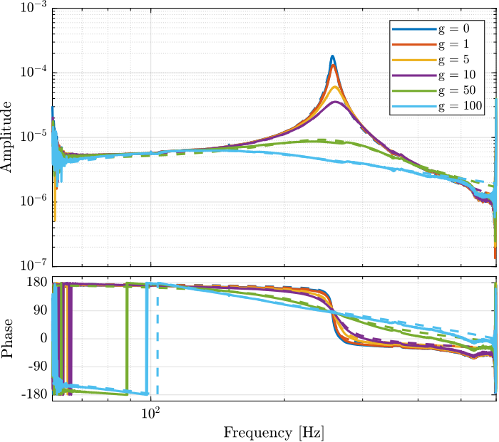
Figure 26: Comparison of the measured dynamic and the identified 2nd order resonant systems that best fits the data
Finally, we can represent the position of the poles of the 2nd order systems on the Root Locus plot (Figure 27).
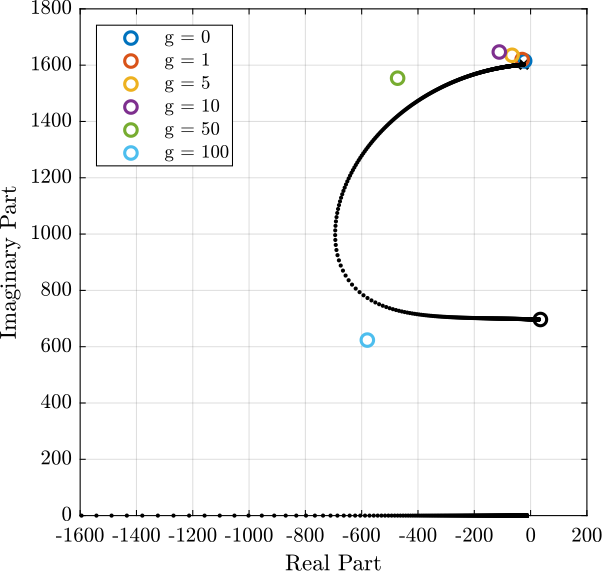
Figure 27: Root Locus plot of the identified IFF plant as well as the identified poles of the damped system