Spectral Analysis using Matlab
Table of Contents
- 1. Spectral Analysis - Basics
- 1.1. Sensitivity of the instrumentation
- 1.2. Convert the time domain from volts to velocity
- 1.3. Power Spectral Density and Amplitude Spectral Density
- 1.4. Modification of a signal’s Power Spectral Density when going through an LTI system
- 1.5. From PSD of the velocity to the PSD of the displacement
- 1.6. Cumulative Power/Amplitude Spectrum
- 2. Time domain signal that approximate a PSD - TF technique
- 3. Time domain signal that approximate a PSD - IFFT technique
- 4. Compute the Noise level and Signal level from PSD
- 5. Further Notes
This document presents the mathematics as well as the matlab scripts to do various spectral analysis on a measured signal.
Some matlab documentation about Spectral Analysis can be found here.
First, in section 1, some basics of spectral analysis are presented.
In some cases, we want to generate a time domain signal with defined Power Spectral Density. Two methods are presented in sections 2 and 3.
Finally, some notes are done on how to compute the noise level and signal level from a given Power Spectral Density in section 4.
1 Spectral Analysis - Basics
In this section, the basics of spectral analysis is presented with the associated Matlab commands.
This include:
- how to compute the Power Spectral Density (PSD) and the Amplitude Spectral Density (ASD)
- how to take into account the sensitivity of the sensor and of the electronics
- how to compute the Cumulative Power Spectrum (CPS) and the Cumulative Amplitude Spectrum (CAS)
1.1 Sensitivity of the instrumentation
A typical measurement setup is shown in figure 1 where we measure a physical signal which is here a velocity \(v(t)\) using a geophone. The geophone has some dynamics that we represent with \(G_g(s)\), its output a voltage. The output of the geophone is then amplified by a voltage amplifier with a transfer function \(G_a(s)\).
Finally, the signal is discretised with an ADC and we obtain \(x(k\Delta t)\).
To obtain the real physical quantity \(v(t)\) as measured by the sensor from the obtained signal \(x(k\Delta t)\), one have to know the sensitivity of the sensors and electronics used (\(G_g(s)\) and \(G_a(s)\)).
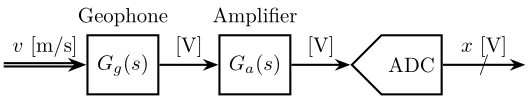
Figure 1: Schematic of the instrumentation used for the measurement
Let’s say, we know that the sensitivity of the geophone used is \[ G_g(s) = G_0 \frac{\frac{s}{2\pi f_0}}{1 + \frac{s}{2\pi f_0}} \quad \left[\frac{V}{m/s}\right] \]
The parameters are defined below.
  G0 = 88; % Sensitivity [V/(m/s)]
  f0 = 2; % Cut-off frequency [Hz]

  Gg = G0*(s/2/pi/f0)/(1+s/2/pi/f0);
And the dynamics of the amplifier in the bandwidth of interest is just a gain: \(G_a(s) = 1000\).
Ga = 1000;
1.2 Convert the time domain from volts to velocity
Let’s here try to obtain the time domain signal \(v(t)\) from the measurement \(x\).
If \({G_a(s)}^{-1} {G_g(s)}^{-1}\) is proper, we can simulate this dynamical system to go from the voltage \(x\) to the velocity \(v\) as shown in figure 2.
If \({G_a(s)}^{-1} {G_g(s)}^{-1}\) is not proper, we add low pass filters at high frequency to make the system proper.
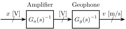
Figure 2: Schematic of the instrumentation used for the measurement
Let’s load the measured \(x\).
  data = load('mat/data_028.mat', 'data'); data = data.data;

  t = data(:, 3); % Time vector [s]
  x = data(:, 1)-mean(data(:, 1)); % The offset if removed (coming from the voltage amplifier) [v]

  dt = t(2)-t(1); % Sampling Time [s]
  Fs = 1/dt; % Sampling Frequency [Hz]
We simulate this system with matlab using the lsim command.
v = lsim(inv(Gg*Ga), x, t);
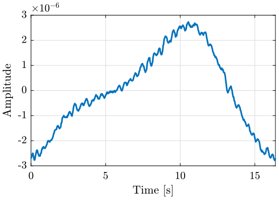
And we plot the obtained velocity
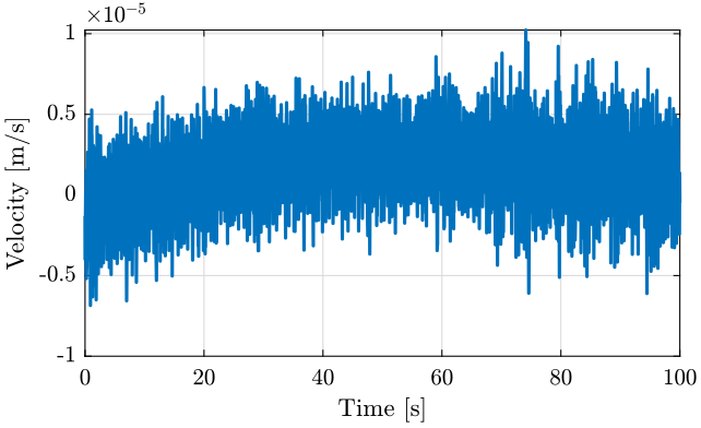
Figure 3: Computed Velocity from the measured Voltage
1.3 Power Spectral Density and Amplitude Spectral Density
From the Matlab documentation:
The goal of spectral estimation is to describe the distribution (over frequency) of the power contained in a signal, based on a finite set of data.
We now have the velocity \(v(t)\ [m/s]\) in the time domain.
The Power Spectral Density (PSD) \(S_v(f)\) of the time domain \(v(t)\) can be computed using the following equation: \[ S_v(f) = \frac{1}{f_s} \sum_{m=-\infty}^{\infty} R_{xx}(m) e^{-j 2 \pi m f / f_s} \ \left[\frac{(m/s)^2}{Hz}\right] \] where
- \(f_s\) is the sampling frequency in Hz
- \(R_{xx}\) is the autocorrelation
The PSD represents the distribution of the (average) signal power over frequency. \(S_v(f)df\) is the infinitesimal power in the band \((f-df/2, f+df/2)\) and the total power in the signal is obtained by integrating these infinitesimal contributions.
To compute the Power Spectral Density with matlab, we use the pwelch function (documentation).
The use of the pwelch function is:
[pxx,w] = pwelch(x,window,noverlap,nfft, fs)
with:
xis the discrete time signalwindowis a window that is used to smooth the obtained PSDoverlapcan be used to have some overlap from section to sectionnfftspecifies the number of FFT points for the PSDfsis the sampling frequency of the dataxin Hertz
As explained in (Schmid 2012), it is recommended to use the pwelch function the following way:
First, define a window (preferably the hanning one) by specifying the averaging factor na.
  nx = length(v);
  na = 8;
  win = hanning(floor(nx/na));
Then, compute the power spectral density \(S_v\) and the associated frequency vector \(f\) with no overlap.
[Sv, f] = pwelch(v, win, 0, [], Fs);
The obtained PSD is shown in figure 4.

Figure 4: Power Spectral Density of the measured velocity
The Amplitude Spectral Density (ASD) is defined as the square root of the Power Spectral Density and is shown in figure 5.
\begin{equation} \Gamma_{vv}(f) = \sqrt{S_{vv}(f)} \quad \left[ \frac{m/s}{\sqrt{Hz}} \right] \end{equation}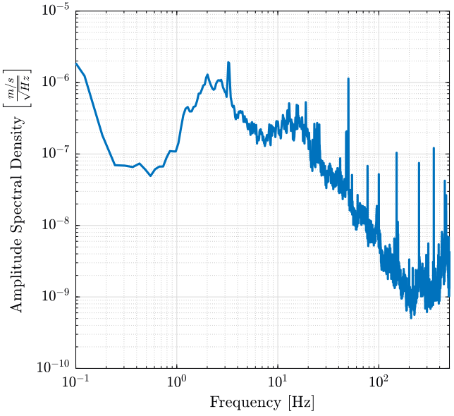
Figure 5: Power Spectral Density of the measured velocity
1.4 Modification of a signal’s Power Spectral Density when going through an LTI system
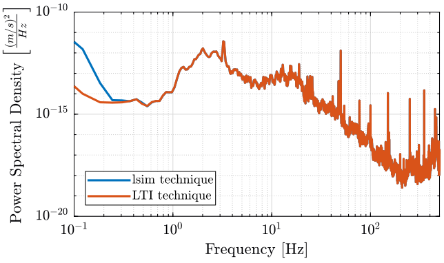
Instead of computing the time domain velocity before computing the Power Spectral Density, we could have directly computed the PSD of the measured voltage \(x\) and then take into account the sensitivity of the measurement devices to have the PSD of the velocity.
To do so, we use the fact that a signal \(u\) with a PSD \(S_{uu}\) going through a LTI system \(G_(s)\) (figure 6) will generate a signal \(y\) with a PSD:
\begin{equation} S_{yy}(\omega) = \left|G(j\omega)\right|^2 S_{uu}(\omega) \end{equation}
Figure 6: Schematic of the instrumentation used for the measurement
Similarly, the ASD of \(y\) is:
\begin{equation} \Gamma_{yy}(\omega) = \left|G(j\omega)\right| \Gamma_{uu}(\omega) \end{equation}Thus, we could have computed the PSD of \(x\) and then obtain the PSD of the velocity with: \[ S_{v}(\omega) = |G_a(j\omega) G_g(j\omega)|^{-1} S_{x}(\omega) \]
The PSD of \(x\) is computed below.
  nx = length(x);
  na = 8;
  win = hanning(floor(nx/na));
  [Sx, f] = pwelch(x, win, 0, [], Fs);
And the PSD of \(v\) is obtained with the below code.
Svv = Sx.*squeeze(abs(freqresp(inv(Gg*Ga), f, 'Hz'))).^2;
The result is compare with the PSD computed from the \(v\) signal obtained with the lsim command in figure 7.
1.5 From PSD of the velocity to the PSD of the displacement
Similarly to what has been done in the last section, we can consider the displacement \(d\) can be obtained from the velocity \(v\) by going through an LTI system \(1/s\) as shown in figure 8.

Figure 8: Schematic of the instrumentation used for the measurement
We then have the relation between the PSD of \(d\) and the PSD of \(v\):
\begin{equation} S_{dd}(\omega) = \left|\frac{1}{j \omega}\right|^2 S_{vv}(\omega) \end{equation}Using a frequency variable \(f\) in Hz:
\begin{equation} S_{dd}(f) = \left| \frac{1}{j 2\pi f} \right|^2 S_{vv}(f) \end{equation}For the Amplitude Spectral Density:
\begin{equation} \Gamma_{dd}(f) = \frac{1}{2\pi f} \Gamma_{vv}(f) \end{equation}Note here that the PSD (and ASD) of one variable and its derivatives/integrals are equal at one particular frequency \(f = 1\ rad/s \approx 0.16\ Hz\):
\begin{equation} S_{xx}(\omega = 1) = S_{vv}(\omega = 1) \end{equation}With Matlab, the PSD of the displacement can be computed from the PSD of the velocity with the following code.
Sd = Sv.*(1./(2*pi*f)).^2;
The obtained PSD of the displacement can be seen in figure 9.

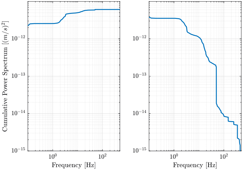
1.6 Cumulative Power/Amplitude Spectrum
The Cumulative Power Spectrum is the cumulative integral of the Power Spectral Density:
\begin{equation} \label{org644886e} CPS_v(f) = \int_0^f PSD_v(\nu) d\nu \quad [(m/s)^2] \end{equation}It is also possible to integrate from high frequency to low frequency:
\begin{equation} \label{org47d268d} CPS_v(f) = \int_f^\infty PSD_v(\nu) d\nu \quad [(m/s)^2] \end{equation}The Cumulative Power Spectrum taken at frequency \(f\) thus represent the power in the signal in the frequency band \(0\) to \(f\) or \(f\) to \(\infty\) depending on the above definition taken.
The choice of the integral direction depends on the shape of the PSD. If the power is mostly present at low frequencies, it is preferable to use equation \eqref{org47d268d}.
The Cumulative Amplitude Spectrum is defined as the square root of the Cumulative Power Spectrum: \[ CAS_v(f) = \sqrt{CPS_v(f)} = \sqrt{\int_f^\infty PSD_v(\nu) d\nu} \quad [m/s] \]
The Root Mean Square value of the velocity corresponds to the Cumulative Amplitude Spectrum when integrated at all frequencies: \[ v_{\text{rms}} = \sqrt{\int_0^\infty PSD_v(\nu) d\nu} = CAS_v(0) \quad [m/s \ \text{rms}] \]
With Matlab, the Cumulative Power Spectrum can be computed with the below formulas and the results are shown in figure 10.
  CPS_v  = cumtrapz(f, Sv); % Cumulative Power Spectrum from low to high frequencies
  CPS_vv = flip(-cumtrapz(flip(f), flip(Sv))); % Cumulative Power Spectrum from high to low frequencies
  figure;
  ax1 = subplot(1, 2, 1);
  hold on;
  plot(f, CPS_v);
  hold off;
  set(gca, 'xscale', 'log'); set(gca, 'yscale', 'log');
  xlabel('Frequency [Hz]'); ylabel('Cumulative Power Spectrum [$(m/s)^2$]')

  ax2 = subplot(1, 2, 2);
  hold on;
  plot(f, CPS_vv);
  hold off;
  set(gca, 'xscale', 'log'); set(gca, 'yscale', 'log');
  xlabel('Frequency [Hz]');

  linkaxes([ax1,ax2],'xy');
  xlim([0.1, 500]); ylim([1e-15, 1e-11]);
2 Time domain signal that approximate a PSD - TF technique
2.1 Signal’s PSD
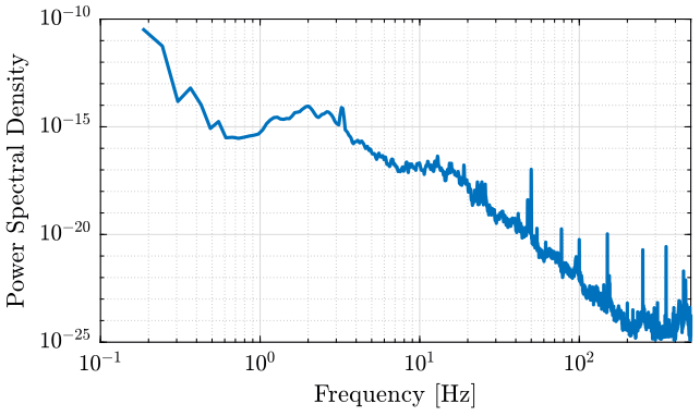
We load the PSD of the signal we wish to replicate.
load('./mat/dist_psd.mat', 'dist_f');
We remove the first value with very high PSD.
  dist_f.f = dist_f.f(3:end);
  dist_f.psd_gm = dist_f.psd_gm(3:end);
The PSD of the signal is shown on figure fig:psd_ground_motion.

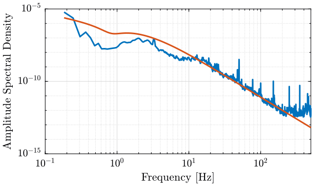
2.2 Transfer Function that approximate the ASD
Using sisotool or any other tool, we create a transfer function \(G\) such that its magnitude is close to the Amplitude Spectral Density \(\Gamma_x = \sqrt{S_x}\):
\[ |G(j\omega)| \approx \Gamma_x(\omega) \]
G_gm = 0.002*(s^2 + 3.169*s + 27.74)/(s*(s+32.73)*(s+8.829)*(s+7.983)^2);
We compare the ASD \(\Gamma_x(\omega)\) and the magnitude of the generated transfer function \(|G(j\omega)|\) in figure 12.
2.3 Generated Time domain signal
We know that a signal \(u\) going through a LTI system \(G\) (figure 13) will have its ASD modified according to the following equation:
\begin{equation} \Gamma_{yy}(\omega) = \left|G(j\omega)\right| \Gamma_{uu}(\omega) \end{equation}
Figure 13: Schematic of the instrumentation used for the measurement
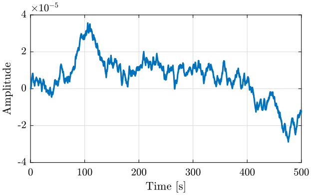
Thus, if we create a random signal with an ASD equal to one at all frequency and we pass this signal through the previously defined LTI transfer function G_gm, we should obtain a signal with an ASD that approximate the original ASD.
To obtain a random signal with an ASD equal to one, we use the following code.
  Fs = 2*dist_f.f(end); % Sampling Frequency [Hz]
  Ts = 1/Fs; % Sampling Time [s]

  t = 0:Ts:500; % Time Vector [s]
  u = sqrt(Fs/2)*randn(length(t), 1); % Signal with an ASD equal to one
We then use lsim to compute \(y\) as shown in figure 13.
y = lsim(G_gm, u, t);
The obtained time domain signal is shown in figure 14.
2.4 Comparison of the Power Spectral Densities
We now compute the Power Spectral Density of the computed time domain signal \(y\).
  nx = length(y);
  na = 16;
  win = hanning(floor(nx/na));

  [pxx, f] = pwelch(y, win, 0, [], Fs);
Finally, we compare the PSD of the original signal and the obtained signal on figure fig:psd_comparison.
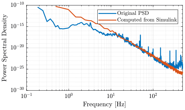
2.5 Simulink
One advantage of this technique is that it can be easily integrated into simulink.
The corresponding schematic is shown in figure 16 where the block Band-Limited White Noise is used to generate a random signal with a PSD equal to one (parameter Noise Power is set to 1).
Then, the signal generated pass through the transfer function representing the wanted ASD.
Figure 16: Simulink Schematic
We simulate the system shown in figure 16.
out = sim('matlab/generate_signal_psd.slx');
And we compute the PSD of the generated signal.
  nx = length(out.u_gm.Data);
  na = 8;
  win = hanning(floor(nx/na));

  [pxx, f] = pwelch(out.u_gm.Data, win, 0, [], 1e3);
Finally, we compare the PSD of the generated signal with the original PSD in figure 17.
3 Time domain signal that approximate a PSD - IFFT technique
The technique comes from (Preumont 1994) (section 12.11). It is used to compute a periodic signal that has any Power Spectral Density defined. It makes used of the Unversed Fast Fourier Transform (IFFT).
3.1 Signal’s PSD
We load the PSD of the signal we wish to replicate.
load('./mat/dist_psd.mat', 'dist_f');
We remove the first value with very high PSD.
  dist_f.f = dist_f.f(3:end);
  dist_f.psd_gm = dist_f.psd_gm(3:end);
The PSD of the signal is shown on figure fig:psd_original.
3.2 Algorithm
We define some parameters that will be used in the algorithm.
  Fs = 2*dist_f.f(end);    % Sampling Frequency of data is twice the maximum frequency of the PSD vector [Hz]
  N  = 2*length(dist_f.f); % Number of Samples match the one of the wanted PSD
  T0 = N/Fs;               % Signal Duration [s]
  df = 1/T0;               % Frequency resolution of the DFT [Hz]
                           % Also equal to (dist_f.f(2)-dist_f.f(1))
We then specify the wanted PSD.
phi = dist_f.psd_gm;
We create amplitudes corresponding to wanted PSD.
  C = zeros(N/2,1);
  for i = 1:N/2
    C(i) = sqrt(phi(i)*df);
  end
Finally, we add some random phase to C.
  theta = 2*pi*rand(N/2,1); % Generate random phase [rad]

  Cx = [0 ; C.*complex(cos(theta),sin(theta))];
  Cx = [Cx; flipud(conj(Cx(2:end)))];;
3.3 Obtained Time Domain Signal
The time domain data is generated by an inverse FFT.
The ifft Matlab does not take into account the sampling frequency, thus we need to normalize the signal.
  u = N/sqrt(2)*ifft(Cx); % Normalisation of the IFFT
  t = linspace(0, T0, N+1); % Time Vector [s]
3.4 PSD Comparison
We duplicate the time domain signal to have a longer signal and thus a more precise PSD result.
u_rep = repmat(u, 10, 1);
We compute the PSD of the obtained signal with the following commands.
  nx = length(u_rep);
  na = 16;
  win = hanning(floor(nx/na));

  [pxx, f] = pwelch(u_rep, win, 0, [], Fs);
Finally, we compare the PSD of the original signal and the obtained signal on figure fig:psd_comparison.

4 Compute the Noise level and Signal level from PSD
We here make use of the Power Spectral Density to estimate either the noise level or the amplitude of a deterministic signal. Everything is explained in (Schmid 2012) sections 5 and 6.
4.1 Time Domain Signal
Let’s first define the number of sample and the sampling time.
  N  = 10000; % Number of Sample
  dt = 0.001; % Sampling Time [s]

  t = dt*(0:1:N-1)'; % Time vector [s]
We generate of signal that consist of:
- a white noise with an RMS value equal to
anoi - two sinusoidal signals
The parameters are defined below.
  asig = 0.1; % Amplitude of the signal [V]
  fsig = 10;  % Frequency of the signal [Hz]

  ahar = 0.5; % Amplitude of the harmonic [V]
  fhar = 50;  % Frequency of the harmonic [Hz]

  anoi = 1e-3; % RMS value of the noise
The signal \(x\) is generated with the following code and is shown in figure 21.
x = anoi*randn(N, 1) + asig*sin((2*pi*fsig)*t) + ahar*sin((2*pi*fhar)*t);
4.2 Estimation of the magnitude of a deterministic signal
Let’s compute the PSD of the signal using the blackmanharris window.
  nx = length(x);
  na = 8;
  win = blackmanharris(floor(nx/na));

  [pxx, f] = pwelch(x, win, 0, [], 1/dt);
Normalization of the PSD.
  CG = sum(win)/(nx/na);
  NG = sum(win.^2)/(nx/na);
  fbin = f(2) - f(1);

  pxx_norm = pxx*(NG*fbin/CG^2);
We determine the frequency bins corresponding to the frequency of the signals.
  isig = round(fsig/fbin)+1;
  ihar = round(fhar/fbin)+1;
The theoretical RMS value of the signal is:
srmt = asig/sqrt(2); % Theoretical value of signal magnitude
And we estimate the RMS value of the signal by either integrating the PSD around the frequency of the signal or by just taking the maximum value.
  srms = sqrt(sum(pxx(isig-5:isig+5)*fbin)); % Signal spectrum integrated
  srmsp = sqrt(pxx_norm(isig) * NG*fbin/CG^2); % Maximum read off spectrum
| Signal Magnitude [rms] | |
|---|---|
| Theoretical | 0.0707 |
| Integrated | 0.0707 |
| Maximum | 0.0529 |
We see that the integrated value gives a good approximate of the true RMS value whereas the maximum value give an poor approximate. This effect is called scallop loss. Thus, always the integrated method should be used.
4.3 Estimation of the noise level
The noise level can also be computed using the integration method.
The theoretical RMS noise value is.
nth = anoi/sqrt(max(f)) % Theoretical value [V/sqrt(Hz)]
We can estimate this RMS value by integrating the PSD at frequencies where the power of the noise signal is above the power of the other signals.
navg = sqrt(mean(pxx_norm([ihar+10:end]))) % pwelch output averaged
| test | |
|---|---|
| Theoretical | 4.472e-05 |
| Average | 4.337e-05 |
The estimate of the noise level is quite good.
5 Further Notes
5.1 PSD of ADC quantization noise
This is taken from here.
Let’s note:
- \(q\) is the corresponding value in [V] of the least significant bit (LSB)
- \(\Delta V\) is the full range of the ADC in [V]
- \(n\) is the number of ADC’s bits
- \(f_s\) is the sample frequency in [Hz]
Let’s suppose that the ADC is ideal. The only noise comes from the quantization error. Interestingly, the noise amplitude is uniformly distributed.
The quantization noise can take a value between \(\pm q/2\), and the probability density function is constant in this range (i.e., it’s a uniform distribution). Since the integral of the probability density function is equal to one, its value will be \(1/q\) for \(-q/2 < e < q/2\) (Fig. 22).
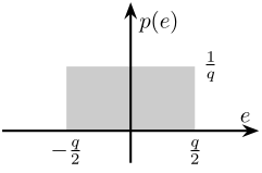
Figure 22: Probability density function \(p(e)\) of the ADC error \(e\)
Now, we can calculate the time average power of the quantization noise as
\begin{equation} P_q = \int_{-q/2}^{q/2} e^2 p(e) de = \frac{q^2}{12} \end{equation}The other important parameter of a noise source is the power spectral density (PSD), which indicates how the noise power spreads in different frequency bands. To find the power spectral density, we need to calculate the Fourier transform of the autocorrelation function of the noise.
Assuming that the noise samples are not correlated with one another, we can approximate the autocorrelation function with a delta function in the time domain. Since the Fourier transform of a delta function is equal to one, the power spectral density will be frequency independent. Therefore, the quantization noise is white noise with total power equal to \(P_q = \frac{q^2}{12}\).
Thus, the two-sided PSD (from \(\frac{-f_s}{2}\) to \(\frac{f_s}{2}\)), we should divide the noise power \(P_q\) by \(f_s\):
\begin{equation} \int_{-f_s/2}^{f_s/2} \Gamma(f) d f = f_s \Gamma = \frac{q^2}{12} \end{equation}Finally:
\begin{equation} \begin{aligned} \Gamma &= \frac{q^2}{12 f_s} \\ &= \frac{\left(\frac{\Delta V}{2^n}\right)^2}{12 f_s} \text{ in } \left[ \frac{V^2}{Hz} \right] \end{aligned} \end{equation}