Static Measurements

1. Measurement description
2. Static measurement of the translation stage
3. Static Measurement of the spindle

1 Measurement description

Setup: Each stage is statically moved of all its stroke on after the other. A metrology element is located at the sample position and its motion is measured in translations and rotations. For each small displacement, the stage is stopped and the motion of the sample is recorded and averaged.

The report by H-P van der Kleij on the static measurement of the ID31 station is available here.

Date	2019-01-09
Sensors	Interferometer
Location	Experimental Hutch

Goal: The goal here is to analyze the static measurement on the station (guiding error of each stage) and convert them to dynamic disturbances that can be use in the model of the micro-station.

2 Static measurement of the translation stage

All the files (data and Matlab scripts) are accessible here.

2.1 Notes

5530: Straightness Plot: Yz
Filename: r:\home\PDMU\PEL\Measurement_library\ID31\ID31_u_station\TY\12_12_2018\linear deviation _tyz_401_points.txt
Acquisition date: 09/01/2019 13:49:42
Current date: 08/03/2019 08:46:35
Measurement Type: STRAIGHTNESS vertical
Travel Mode: Bidirectional
Number of Target Positions: 401
Number of total data pairs: 2406
Number of total data runs:6
Position Value Units: millimeters
Error Value Units: micrometers

Environmental Data	Min	Max	Avg
Air Temp (C)	024,57	024,61	024,59
Air Prs (mm)	742,56	743,29	742,83
Air Hmd (%)	024,00	024,00	024,00
MT1 Temp (C)			020,00
MT2 Temp (C)	024,40	024,44	024,42
MT3 Temp (C)	024,32	024,36	024,34

In a very schematic way, the measurement is explained on figure 1. The positioning error \(d\) is measure as a function of \(x\). Because the measurement is done in a static way, the dynamics of the station (represented by the mass-spring-damper system on the schematic) does not play a role in the measure.

The obtained data corresponds to the guiding errors.

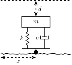
Figure 1: Schematic of the measurement

2.2 Data Pre-processing

sed 's/\t/  /g;s/\,/./g' "mat/linear_deviation_tyz_401_points.txt" > mat/data_tyz.txt

head "mat/data_tyz.txt"

Run	Pos	TargetValue	ErrorValue
1	1	-4.5E+00	7.5377892E+00
1	2	-4.4775E+00	7.5422246E+00
1	3	-4.455E+00	7.5655617E+00
1	4	-4.4325E+00	7.5149518E+00
1	5	-4.41E+00	7.4886377E+00
1	6	-4.3875E+00	7.437007E+00
1	7	-4.365E+00	7.4449354E+00
1	8	-4.3425E+00	7.3937387E+00
1	9	-4.32E+00	7.3287468E+00

2.3 Matlab - Data Import

filename = 'mat/data_tyz.txt';
fileID = fopen(filename);
data = cell2mat(textscan(fileID,'%f  %f  %f  %f', 'collectoutput', 1,'headerlines',1));
fclose(fileID);

2.4 Data - Plot

First, we plot the straightness error as a function of the position (figure 2).

figure;
hold on;
for i=1:data(end, 1)
  plot(data(data(:, 1) == i, 3), data(data(:, 1) == i, 4), '-k');
end
hold off;
xlabel('Target Value [mm]'); ylabel('Error Value [$\mu m$]');

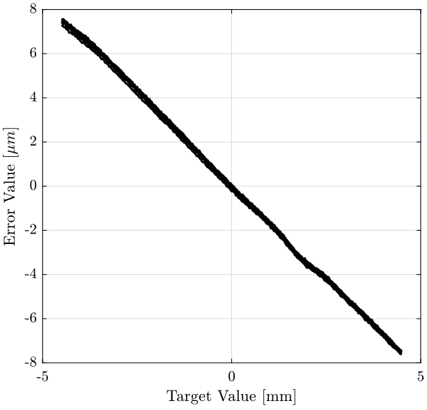
Figure 2: Time domain Data

Then, we compute mean value of each position, and we remove this mean value from the data. The results are shown on figure 3.

mean_pos = zeros(sum(data(:, 1)==1), 1);
for i=1:sum(data(:, 1)==1)
  mean_pos(i) = mean(data(data(:, 2)==i, 4));
end

figure;
hold on;
for i=1:data(end, 1)
  filt = data(:, 1) == i;
  plot(data(filt, 3), data(filt, 4) - mean_pos, '-k');
end
hold off;
xlabel('Target Value [mm]'); ylabel('Error Value [$\mu m$]');

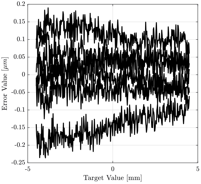
Figure 3: caption

2.5 Translate to time domain

We here make the assumptions that, during a scan with the translation stage, the Z motion of the translation stage will follow the guiding error measured.

We then create a time vector \(t\) from 0 to 1 second that corresponds to a typical scan, and we plot the guiding error as a function of the time on figure 4.

t = linspace(0, 1, length(data(data(:, 1)==1, 4)));

figure;
hold on;
plot(t, data(data(:, 1) == 1, 4) - mean_pos, '-k');
hold off;
xlabel('Time [s]'); ylabel('Error Value [um]');

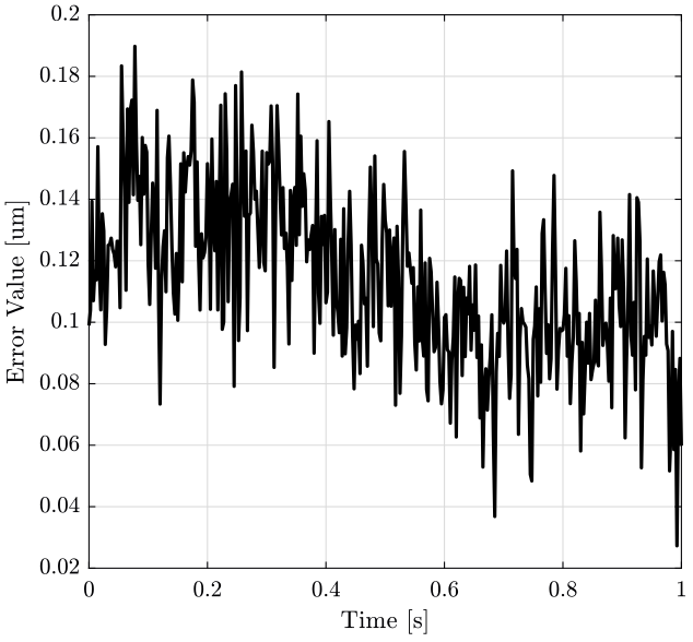
Figure 4: caption

2.6 Compute the PSD

We first compute some parameters that will be used for the PSD computation.

dt = t(2)-t(1);

Fs = 1/dt; % [Hz]

win = hanning(ceil(1*Fs));

We remove the mean position from the data.

x = data(data(:, 1) == 1, 4) - mean_pos;

And finally, we compute the power spectral density of the displacement obtained in the time domain.

The result is shown on figure 5.

[pxx, f] = pwelch(x, win, [], [], Fs);

pxx_t = zeros(length(pxx), data(end, 1));

for i=1:data(end, 1)
  x = data(data(:, 1) == i, 4) - mean_pos;
  [pxx, f] = pwelch(x, win, [], [], Fs);
  pxx_t(:, i) = pxx;
end

figure;
hold on;
plot(f, sqrt(mean(pxx_t, 2)), 'k-');
hold off;
xlabel('Frequency (Hz)');
ylabel('Amplitude Spectral Density $\left[\frac{m}{\sqrt{Hz}}\right]$');
set(gca, 'XScale', 'log'); set(gca, 'YScale', 'log');

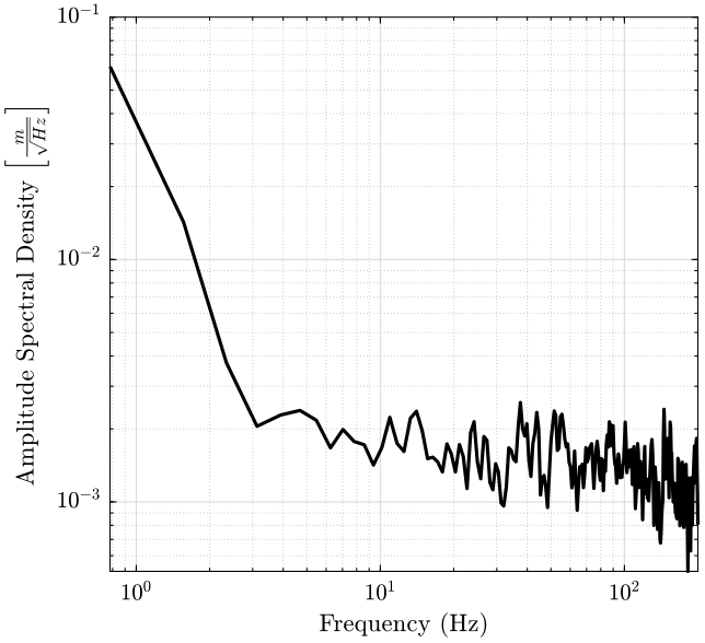
Figure 5: PSD of the Z motion when scanning with Ty at 1Hz

3 Static Measurement of the spindle