Spindle Analysis
Table of Contents
- 1. Notes
- 2. Data Processing
- 3. Time Domain Data
- 4. Model of the spindle
- 4.1. Schematic of the model
- 4.2. Parameters
- 4.3. Compute Mass and Stiffness Matrices
- 4.4. Compute resonance frequencies
- 4.5. From model_damping compute the Damping Matrix
- 4.6. Define inputs, outputs and state names
- 4.7. Define A, B and C matrices
- 4.8. Generate the State Space Model
- 4.9. Bode Plot
- 4.10. Save the model
- 5. Frequency Domain Data
- 5.1. Load the processed data and the model
- 5.2. Compute the PSD
- 5.3. Plot the computed PSD
- 5.4. Compute the response of the model
- 5.5. Plot the PSD of the Force using the model
- 5.6. Estimated Shape of the PSD of the force
- 5.7. PSD in [N]
- 5.8. PSD in [m]
- 5.9. Compute the resulting RMS value [m]
- 5.10. Compute the resulting RMS value [m]
- 6. Functions
The report made by the PEL is accessible here.
1 Notes
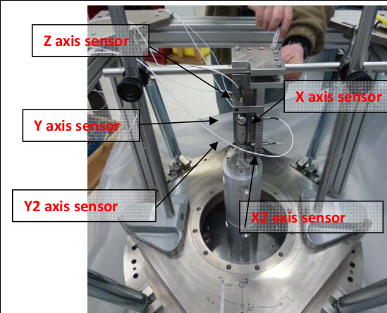
Figure 1: Measurement setup at the PEL lab
| Date | 2017-04-25 |
| Location | PEL Lab |
The goal is to estimate all the error motions induced by the Spindle
2 Data Processing
All the files (data and Matlab scripts) are accessible here.
2.1 Load Measurement Data
spindle_1rpm_table  = readtable('./mat/10turns_1rpm_icepap.txt');
spindle_60rpm_table = readtable('./mat/10turns_60rpm_IcepapFIR.txt');
spindle_1rpm_table(1, :)
spindle_1rpm  = table2array(spindle_1rpm_table);
spindle_60rpm = table2array(spindle_60rpm_table);
2.2 Convert Signals from [deg] to [sec]
speed_1rpm = 360/60; % [deg/sec]
spindle_1rpm(:, 1) = spindle_1rpm(:, 2)/speed_1rpm;  % From position [deg] to time [s]

speed_60rpm = 360/1; % [deg/sec]
spindle_60rpm(:, 1) = spindle_60rpm(:, 2)/speed_60rpm; % From position [deg] to time [s]
2.3 Convert Signals
% scaling = 1/80000; % 80 mV/um
scaling = 1e-6; % [um] to [m]

spindle_1rpm(:, 3:end) = scaling*spindle_1rpm(:, 3:end); % [V] to [m]
spindle_1rpm(:, 3:end) = spindle_1rpm(:, 3:end)-mean(spindle_1rpm(:, 3:end)); % Remove mean

spindle_60rpm(:, 3:end) = scaling*spindle_60rpm(:, 3:end); % [V] to [m]
spindle_60rpm(:, 3:end) = spindle_60rpm(:, 3:end)-mean(spindle_60rpm(:, 3:end)); % Remove mean
2.4 Ts and Fs for both measurements
Ts_1rpm = spindle_1rpm(end, 1)/(length(spindle_1rpm(:, 1))-1);
Fs_1rpm = 1/Ts_1rpm;

Ts_60rpm = spindle_60rpm(end, 1)/(length(spindle_60rpm(:, 1))-1);
Fs_60rpm = 1/Ts_60rpm;
2.5 Find Noise of the ADC [\(\frac{m}{\sqrt{Hz}}\)]
data = spindle_1rpm(:, 5);
dV_1rpm = min(abs(data(1) - data(data ~= data(1))));
noise_1rpm = dV_1rpm/sqrt(12*Fs_1rpm/2);

data = spindle_60rpm(:, 5);
dV_60rpm = min(abs(data(50) - data(data ~= data(50))));
noise_60rpm = dV_60rpm/sqrt(12*Fs_60rpm/2);
2.6 Save all the data under spindle struct
spindle.rpm1.time = spindle_1rpm(:, 1);
spindle.rpm1.deg  = spindle_1rpm(:, 2);
spindle.rpm1.Ts   = Ts_1rpm;
spindle.rpm1.Fs   = 1/Ts_1rpm;
spindle.rpm1.x    = spindle_1rpm(:, 3);
spindle.rpm1.y    = spindle_1rpm(:, 4);
spindle.rpm1.z    = spindle_1rpm(:, 5);
spindle.rpm1.adcn = noise_1rpm;

spindle.rpm60.time = spindle_60rpm(:, 1);
spindle.rpm60.deg  = spindle_60rpm(:, 2);
spindle.rpm60.Ts   = Ts_60rpm;
spindle.rpm60.Fs   = 1/Ts_60rpm;
spindle.rpm60.x    = spindle_60rpm(:, 3);
spindle.rpm60.y    = spindle_60rpm(:, 4);
spindle.rpm60.z    = spindle_60rpm(:, 5);
spindle.rpm60.adcn = noise_60rpm;
2.7 Compute Asynchronous data
for direction = {'x', 'y', 'z'}
    spindle.rpm1.([direction{1}, 'async']) = getAsynchronousError(spindle.rpm1.(direction{1}), 10);
    spindle.rpm60.([direction{1}, 'async']) = getAsynchronousError(spindle.rpm60.(direction{1}), 10);
end
2.8 Save data
save('./mat/spindle_data.mat', 'spindle');
3 Time Domain Data
All the files (data and Matlab scripts) are accessible here.
3.1 Load the processed data
load('./mat/spindle_data.mat', 'spindle');
3.2 Plot X-Y-Z position with respect to Time - 1rpm
figure;
hold on;
plot(spindle.rpm1.time, spindle.rpm1.x);
plot(spindle.rpm1.time, spindle.rpm1.y);
plot(spindle.rpm1.time, spindle.rpm1.z);
hold off;
xlabel('Time [s]'); ylabel('Amplitude [m]');
legend({'tx - 1rpm', 'ty - 1rpm', 'tz - 1rpm'});

Figure 2: Raw time domain translation - 1rpm
3.3 Plot X-Y-Z position with respect to Time - 60rpm
The measurements for the spindle turning at 60rpm are shown figure 3.
figure;
hold on;
plot(spindle.rpm60.time, spindle.rpm60.x);
plot(spindle.rpm60.time, spindle.rpm60.y);
plot(spindle.rpm60.time, spindle.rpm60.z);
hold off;
xlabel('Time [s]'); ylabel('Amplitude [m]');
legend({'tx - 60rpm', 'ty - 60rpm', 'tz - 60rpm'});
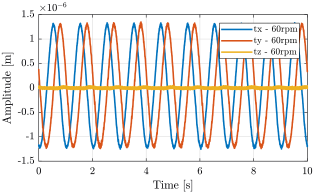
Figure 3: Raw time domain translation - 60rpm
3.4 Plot Synchronous and Asynchronous - 1rpm
figure;
hold on;
plot(spindle.rpm1.time, spindle.rpm1.x);
plot(spindle.rpm1.time, spindle.rpm1.xasync);
hold off;
xlabel('Time [s]'); ylabel('Amplitude [m]');
legend({'tx - 1rpm - Sync', 'tx - 1rpm - Async'});
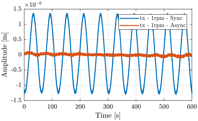
Figure 4: Comparison of the synchronous and asynchronous displacements - 1rpm
3.5 Plot Synchronous and Asynchronous - 60rpm
The data is split into its Synchronous and Asynchronous part (figure 5). We then use the Asynchronous part for the analysis in the following sections as we suppose that we can deal with the synchronous part with feedforward control.
figure;
hold on;
plot(spindle.rpm60.time, spindle.rpm60.x);
plot(spindle.rpm60.time, spindle.rpm60.xasync);
hold off;
xlabel('Time [s]'); ylabel('Amplitude [m]');
legend({'tx - 60rpm - Sync', 'tx - 60rpm - Async'});
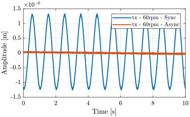
Figure 5: Comparison of the synchronous and asynchronous displacements - 60rpm
3.6 Plot X against Y
figure;
hold on;
plot(spindle.rpm1.x, spindle.rpm1.y);
plot(spindle.rpm60.x, spindle.rpm60.y);
hold off;
xlabel('X Amplitude [m]'); ylabel('Y Amplitude [m]');
legend({'1rpm', '60rpm'});
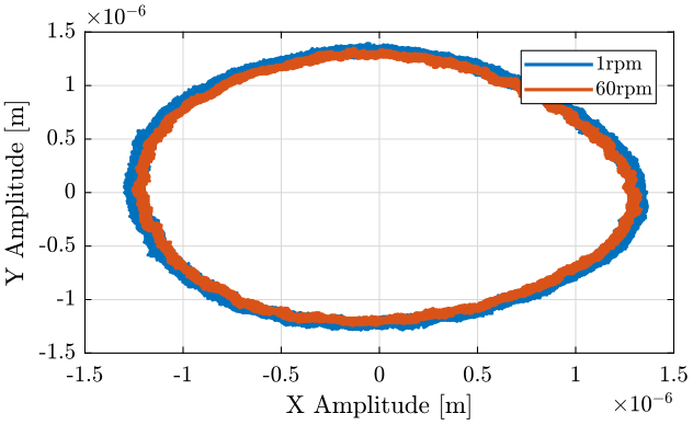
Figure 6: Synchronous x-y displacement
3.7 Plot X against Y - Asynchronous
figure;
hold on;
plot(spindle.rpm1.xasync, spindle.rpm1.yasync);
plot(spindle.rpm60.xasync, spindle.rpm60.yasync);
hold off;
xlabel('X Amplitude [m]'); ylabel('Y Amplitude [m]');
legend({'1rpm', '60rpm'});
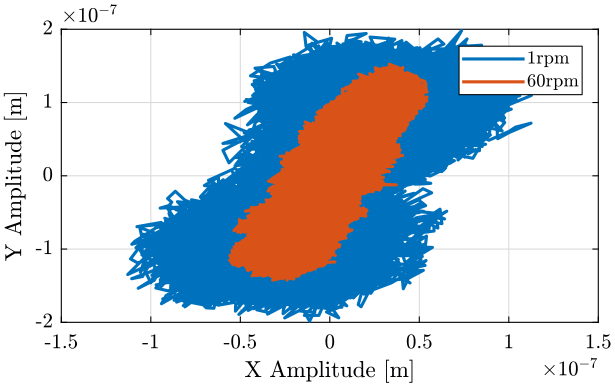
Figure 7: Asynchronous x-y displacement
4 Model of the spindle
All the files (data and Matlab scripts) are accessible here.
4.1 Schematic of the model
The model of the spindle used is shown figure 8.
\(f\) is the perturbation force of the spindle and \(d\) is the measured displacement.
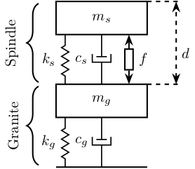
Figure 8: Model of the Spindle
4.2 Parameters
mg = 3000; % Mass of granite [kg]
ms = 50;   % Mass of Spindle [kg]

kg = 1e8; % Stiffness of granite [N/m]
ks = 5e7; % Stiffness of spindle [N/m]
4.3 Compute Mass and Stiffness Matrices
Mm = diag([ms, mg]);
Km = diag([ks, ks+kg]) - diag(ks, -1) - diag(ks, 1);
4.4 Compute resonance frequencies
A = [zeros(size(Mm)) eye(size(Mm)) ; -Mm\Km zeros(size(Mm))];
eigA = imag(eigs(A))/2/pi;
eigA = eigA(eigA>0);
eigA = eigA(1:2);
4.5 From model_damping compute the Damping Matrix
modal_damping = 1e-5;

ab = [0.5*eigA(1) 0.5/eigA(1) ; 0.5*eigA(2) 0.5/eigA(2)]\[modal_damping ; modal_damping];

Cm = ab(1)*Mm +ab(2)*Km;
4.6 Define inputs, outputs and state names
StateName = {...
    'xs', ... % Displacement of Spindle [m]
    'xg', ... % Displacement of Granite [m]
    'vs', ... % Velocity of Spindle [m]
    'vg', ... % Velocity of Granite [m]
            };
StateUnit = {'m', 'm', 'm/s', 'm/s'};

InputName = {...
    'f' ... % Spindle Force [N]
            };
InputUnit = {'N'};

OutputName = {...
    'd' ... % Displacement [m]
             };
OutputUnit = {'m'};
4.7 Define A, B and C matrices
% A Matrix
A = [zeros(size(Mm)) eye(size(Mm)) ; ...
     -Mm\Km          -Mm\Cm];

% B Matrix
B_low = zeros(length(StateName), length(InputName));
B_low(strcmp(StateName,'vs'), strcmp(InputName,'f')) =  1;
B_low(strcmp(StateName,'vg'), strcmp(InputName,'f')) = -1;
B = blkdiag(zeros(length(StateName)/2), pinv(Mm))*B_low;

% C Matrix
C = zeros(length(OutputName), length(StateName));
C(strcmp(OutputName,'d'), strcmp(StateName,'xs')) =  1;
C(strcmp(OutputName,'d'), strcmp(StateName,'xg')) = -1;

% D Matrix
D = zeros(length(OutputName), length(InputName));
4.8 Generate the State Space Model
sys = ss(A, B, C, D);
sys.StateName = StateName;
sys.StateUnit = StateUnit;

sys.InputName = InputName;
sys.InputUnit = InputUnit;

sys.OutputName = OutputName;
sys.OutputUnit = OutputUnit;
4.9 Bode Plot
The transfer function from a disturbance force \(f\) to the measured displacement \(d\) is shown figure 9.
freqs = logspace(-1, 3, 1000);

figure;
plot(freqs, abs(squeeze(freqresp(sys('d', 'f'), freqs, 'Hz'))));
set(gca, 'XScale', 'log'); set(gca, 'YScale', 'log');
xlabel('Frequency [Hz]'); ylabel('Amplitude [m/N]');
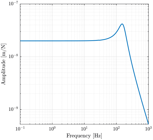
Figure 9: Bode plot of the transfer function from \(f\) to \(d\)
4.10 Save the model
save('./mat/spindle_model.mat', 'sys');
5 Frequency Domain Data
All the files (data and Matlab scripts) are accessible here.
5.1 Load the processed data and the model
load('./mat/spindle_data.mat', 'spindle');
load('./mat/spindle_model.mat', 'sys');
5.2 Compute the PSD
n_av = 4; % Number of average

[pxx_1rpm, f_1rpm] = pwelch(spindle.rpm1.xasync, hanning(ceil(length(spindle.rpm1.xasync)/n_av)), [], [], spindle.rpm1.Fs);
[pyy_1rpm, ~]      = pwelch(spindle.rpm1.yasync, hanning(ceil(length(spindle.rpm1.yasync)/n_av)), [], [], spindle.rpm1.Fs);
[pzz_1rpm, ~]      = pwelch(spindle.rpm1.zasync, hanning(ceil(length(spindle.rpm1.zasync)/n_av)), [], [], spindle.rpm1.Fs);

[pxx_60rpm, f_60rpm] = pwelch(spindle.rpm60.xasync, hanning(ceil(length(spindle.rpm60.xasync)/n_av)), [], [], spindle.rpm60.Fs);
[pyy_60rpm, ~]       = pwelch(spindle.rpm60.yasync, hanning(ceil(length(spindle.rpm60.yasync)/n_av)), [], [], spindle.rpm60.Fs);
[pzz_60rpm, ~]       = pwelch(spindle.rpm60.zasync, hanning(ceil(length(spindle.rpm60.zasync)/n_av)), [], [], spindle.rpm60.Fs);
5.3 Plot the computed PSD
The Amplitude Spectral Densities of the displacement of the spindle for the \(x\), \(y\) and \(z\) directions are shown figure 11. They correspond to the Asynchronous part shown figure 5.
figure;
hold on;
plot(f_1rpm, (pxx_1rpm).^.5, 'DisplayName', '$P_{xx}$ - 1rpm');
plot(f_1rpm, (pyy_1rpm).^.5, 'DisplayName', '$P_{yy}$ - 1rpm');
plot(f_1rpm, (pzz_1rpm).^.5, 'DisplayName', '$P_{zz}$ - 1rpm');
% plot(f_1rpm, spindle.rpm1.adcn*ones(size(f_1rpm)), '--k', 'DisplayName', 'ADC - 1rpm');
hold off;
set(gca, 'XScale', 'log'); set(gca, 'YScale', 'log');
xlabel('Frequency [Hz]'); ylabel('ASD [$m/\sqrt{Hz}$]');
legend('Location', 'northeast');
xlim([f_1rpm(2), f_1rpm(end)]);
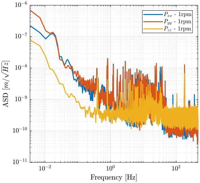
Figure 10: Power spectral density of the Asynchronous displacement - 1rpm
figure;
hold on;
plot(f_60rpm, (pxx_60rpm).^.5, 'DisplayName', '$P_{xx}$ - 60rpm');
plot(f_60rpm, (pyy_60rpm).^.5, 'DisplayName', '$P_{yy}$ - 60rpm');
plot(f_60rpm, (pzz_60rpm).^.5, 'DisplayName', '$P_{zz}$ - 60rpm');
% plot(f_60rpm, spindle.rpm60.adcn*ones(size(f_60rpm)), '--k', 'DisplayName', 'ADC - 60rpm');
hold off;
set(gca, 'XScale', 'log'); set(gca, 'YScale', 'log');
xlabel('Frequency [Hz]'); ylabel('ASD [$m/\sqrt{Hz}$]');
legend('Location', 'northeast');
xlim([f_60rpm(2), f_60rpm(end)]);
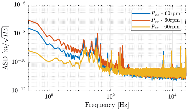
Figure 11: Power spectral density of the Asynchronous displacement - 60rpm
5.4 Compute the response of the model
Tfd = abs(squeeze(freqresp(sys('d', 'f'), f_60rpm, 'Hz')));
5.5 Plot the PSD of the Force using the model
figure;
plot(f_60rpm, (pxx_60rpm.^.5)./Tfd, 'DisplayName', '$P_{xx}$');
set(gca, 'XScale', 'log'); set(gca, 'YScale', 'log');
xlabel('Frequency [Hz]'); ylabel('ASD [$N/\sqrt{Hz}$]');
xlim([f_60rpm(2), f_60rpm(end)]);
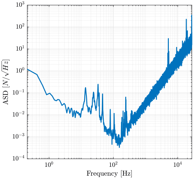
Figure 12: Power spectral density of the force - 60rpm
5.6 Estimated Shape of the PSD of the force
s = tf('s');

Wd_simple = 1e-8/(1+s/2/pi/0.5)/(1+s/2/pi/100);
Wf_simple = Wd_simple/tf(sys('d', 'f'));
TWf_simple = abs(squeeze(freqresp(Wf_simple, f_60rpm, 'Hz')));

% Wf = 0.48902*(s+327.9)*(s^2 + 109.6*s + 1.687e04)/((s^2 + 30.59*s + 8541)*(s^2 + 29.11*s + 3.268e04));
% Wf = 0.15788*(s+418.6)*(s+1697)^2*(s^2 + 124.3*s + 2.529e04)*(s^2 + 681.3*s + 9.018e05)/((s^2 + 23.03*s + 8916)*(s^2 + 33.85*s + 6.559e04)*(s^2 + 71.43*s + 4.283e05)*(s^2 + 40.64*s + 1.789e06));

Wf = (s+1697)^2*(s^2 + 114.5*s + 2.278e04)*(s^2 + 205.1*s + 1.627e05)*(s^2 + 285.8*s + 8.624e05)*(s+100)/((s+0.5)*3012*(s^2 + 23.03*s + 8916)*(s^2 + 17.07*s + 4.798e04)*(s^2 + 41.17*s + 4.347e05)*(s^2 + 78.99*s + 1.789e06));

TWf = abs(squeeze(freqresp(Wf, f_60rpm, 'Hz')));
5.7 PSD in [N]
Above \(200Hz\), the Amplitude Spectral Density seems dominated by noise coming from the electronics (charge amplifier, ADC, …). So we don’t know what is the frequency content of the force above that frequency. However, we assume that \(P_{xx}\) is decreasing with \(1/f\) as it seems so be the case below \(100Hz\) (figure 11).
We then fit the PSD of the displacement with a transfer function (figure 14).
figure;
hold on;
plot(f_60rpm, (pxx_60rpm.^.5)./Tfd, 'DisplayName', '$\sqrt{P_{xx}}/|T_{d/f}|$');
plot(f_60rpm, TWf, 'DisplayName', 'Wf');
plot(f_60rpm, TWf_simple, '-k', 'DisplayName', 'Wfs');
set(gca, 'XScale', 'log'); set(gca, 'YScale', 'log');
xlabel('Frequency [Hz]'); ylabel('ASD [$N/\sqrt{Hz}$]');
xlim([f_60rpm(2), f_60rpm(end)]);
legend('Location', 'northeast');
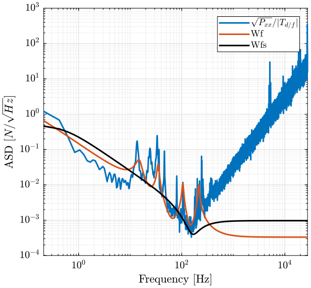
Figure 13: Power spectral density of the force - 60rpm
5.8 PSD in [m]
To obtain the PSD of the force \(f\) that induce such displacement, we use the following formula: \[ \sqrt{PSD(d)} = |T_{d/f}| \sqrt{PSD(f)} \]
And so we have: \[ \sqrt{PSD(f)} = |T_{d/f}|^{-1} \sqrt{PSD(d)} \]
The obtain Power Spectral Density of the force is displayed figure 13.
figure;
hold on;
plot(f_60rpm, pxx_60rpm.^.5, 'DisplayName', '$\sqrt{P_{xx}}$');
plot(f_60rpm, TWf.*Tfd, 'DisplayName', '$|W_f|*|T_{d/f}|$');
set(gca, 'XScale', 'log'); set(gca, 'YScale', 'log');
xlabel('Frequency [Hz]'); ylabel('ASD [$m/\sqrt{Hz}$]');
xlim([f_60rpm(2), f_60rpm(end)]);
legend('Location', 'northeast');
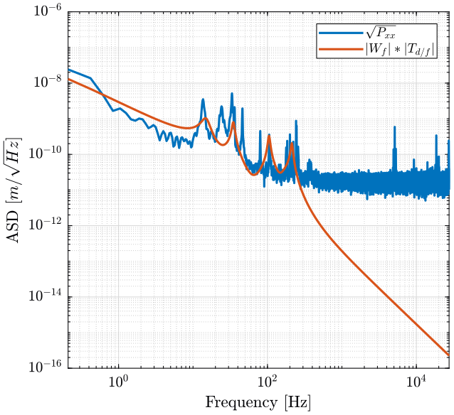
Figure 14: Comparison of the power spectral density of the measured displacement and of the model
5.9 Compute the resulting RMS value [m]
figure;
hold on;
plot(f_60rpm, 1e9*cumtrapz(f_60rpm, (pxx_60rpm)).^.5, '--', 'DisplayName', 'Exp. Data');
plot(f_60rpm, 1e9*cumtrapz(f_60rpm, ((TWf.*Tfd).^2)).^.5, '--', 'DisplayName', 'Estimated');
hold off;
set(gca, 'XScale', 'log');
xlabel('Frequency [Hz]'); ylabel('CPS [$nm$ rms]');
xlim([f_60rpm(2), f_60rpm(end)]);
legend('Location', 'southeast');
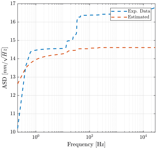
Figure 15: Cumulative Power Spectrum - 60rpm
5.10 Compute the resulting RMS value [m]
figure;
hold on;
plot(f_1rpm, 1e9*cumtrapz(f_1rpm, (pxx_1rpm)), '--', 'DisplayName', 'Exp. Data');
plot(f_1rpm, 1e9*(f_1rpm(end)-f_1rpm(1))/(length(f_1rpm)-1)*cumsum(pxx_1rpm), '--', 'DisplayName', 'Exp. Data');
hold off;
set(gca, 'XScale', 'log');
xlabel('Frequency [Hz]'); ylabel('CPS [$nm$ rms]');
xlim([f_1rpm(2), f_1rpm(end)]);
legend('Location', 'southeast');
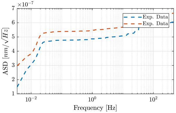
Figure 16: Cumulative Power Spectrum - 1rpm
6 Functions
6.1 getAsynchronousError
This Matlab function is accessible here.
function [Wxdec] = getAsynchronousError(data, NbTurn)
%%
    L = length(data);
    res_per_rev = L/NbTurn;

    P = 0:(res_per_rev*NbTurn-1);
    Pos = P' * 360/res_per_rev;

    % Temperature correction
    x1 = myfit2(Pos, data);

    % Convert data to frequency domain and scale accordingly
    X2 = 2/(res_per_rev*NbTurn)*fft(x1);
    f2 = (0:L-1)./NbTurn; %upr -> once per revolution

    %%
    X2dec = zeros(size(X2));
    % Get only the non integer data
    X2dec(mod(f2(:), 1) ~= 0) = X2(mod(f2(:), 1) ~= 0);

    Wxdec = real((res_per_rev*NbTurn)/2 * ifft(X2dec));

    %%
    function Y =  myfit2(x,y)
        A = [x ones(size(x))]\y;
        a = A(1); b = A(2);
        Y = y - (a*x + b);
    end
end