Ground Motion Measurements

Table of ContentsClose

1. Experimental Setup
2. Measurement Analysis

1 Experimental Setup

The goal here is to compare the ground motion at the location of the micro-station (ID31 beamline at ESRF) with other measurements of the ground motion.

This will also permit to confirm that the device use for the measurement (geophones, amplifiers, ADC) are working well and that the data processing is correct.

One L22 geophone is put on the ID31 floor. The signal is then filtered with a first order low pass filter with a cut-off frequency of $1 k H z$ . Then the signal is amplified by a Voltage Amplifier with the following settings:

AC/DC option set to DC
Amplification of 60dB (1000)
Low pass filter at the output with a cut-off frequency of $1 k H z$

On figure 1 is an overview of multiple measurements made at famous location.

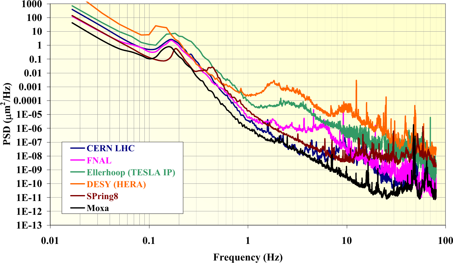
Figure 1: Power spectral density of ground vibration in the vertical direction at multiple locations (source)

2 Measurement Analysis

Note

All the files (data and Matlab scripts) are accessible here.

2.1 Load data

Copy
data = load('mat/data_028.mat', 'data'); data = data.data;

2.2 Time domain plots of the measured voltage

Copy
figure;
hold on;
plot(data(:, 3), data(:, 1));
hold off;
xlabel('Time [s]'); ylabel('Voltage [V]');
xlim([0, 100]);

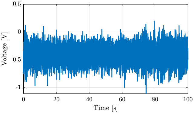
Figure 2: Measurement of the ground motion - Time domain

2.3 Computation of the ASD of the measured voltage

Copy
dt = data(2, 3) - data(1, 3);

Fs = 1/dt;
win = hanning(ceil(10*Fs));

Copy
[px_dc, f] = pwelch(data(:, 1), win, [], [], Fs);

Copy
figure;
hold on;
plot(f, sqrt(px_dc));
hold off;
set(gca, 'xscale', 'log');
set(gca, 'yscale', 'log');
xlabel('Frequency [Hz]'); ylabel('Amplitude Spectral Density $\left[\frac{V}{\sqrt{Hz}}\right]$')
xlim([0.1, 500]);

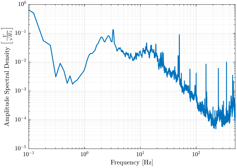
Figure 3: Amplitude Spectral Density of the measured Voltage

2.4 Scaling to take into account the sensibility of the geophone and the voltage amplifier

The Geophone used are L22. Their sensibility is shown on figure 4.

Copy
S0 = 88; % Sensitivity [V/(m/s)]
f0 = 2; % Cut-off frequency [Hz]

S = S0*(s/2/pi/f0)/(1+s/2/pi/f0);

Copy
freqs = logspace(-1, 2, 1000);

figure;
hold on;
plot(f, abs(squeeze(freqresp(S, f, 'Hz'))));
hold off;
set(gca, 'xscale', 'log'); set(gca, 'yscale', 'log');
xlabel('Frequency [Hz]'); ylabel('Magnitude $\left[\frac{V}{m/s}\right]$');
xlim([0.1, 100]);

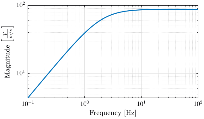
Figure 4: Sensibility of the Geophone

We also take into account the gain of the electronics which is here set to be $60 d B$ .

Copy
G0_db = 60; % [dB]

G0 = 10^(G0_db/20); % [abs]

We divide the PSD measured (in $V^2 / \sqrt{H z}$ ) by the square of the gain of the voltage amplifier to obtain the PSD of the voltage across the geophone. We further divide the result by the square of the magnitude of sensibility of the Geophone to obtain the PSD of the velocity in $(m / s)^{2} / H z$ .

Copy
psd_gv = px_dc./abs(squeeze(freqresp(G0*S, f, 'Hz'))).^2;

Finally, we obtain the PSD of the ground motion in $m^{2} / H z$ by dividing by the square of the frequency in $r a d / s$ .

Copy
psd_gm = psd_gv./(2*pi*f).^2;

2.5 Time domain plots of the ground motion

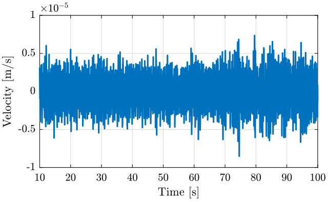
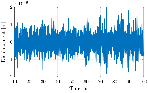
We can inverse the dynamics of the geophone to convert the measured voltage into the estimated ground motion.

Copy
est_vel = lsim(inv(G0*S)*(s/2/pi)/(1+s/2/pi), data(:, 1), data(:, 3)); % Estimated velocity above 1Hz
est_vel = est_vel - mean(est_vel(data(:,3)>10)); % The mean value of the velocity if removed
est_dis = lsim(1/(1+s/2/pi), est_vel, data(:, 3)); % The velocity is integrated above 1Hz

Figure 5: Time domain velocity (png, pdf)

Figure 6: Time domain absolute displacement (png, pdf)

2.6 Computation of the ASD of the velocity and displacement

The ASD of the measured velocity is shown on figure 7.

Copy
figure;
hold on;
plot(f, sqrt(psd_gv));
hold off;
set(gca, 'xscale', 'log');
set(gca, 'yscale', 'log');
xlabel('Frequency [Hz]'); ylabel('ASD of the measured Velocity $\left[\frac{m/s}{\sqrt{Hz}}\right]$')
xlim([0.1, 500]);

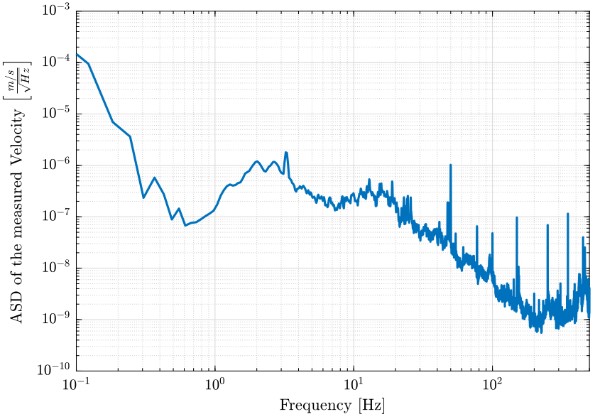
Figure 7: Amplitude Spectral Density of the Velocity

We also plot the ASD in displacement (figure 8);

Copy
figure;
hold on;
plot(f, sqrt(psd_gm));
hold off;
set(gca, 'xscale', 'log'); set(gca, 'yscale', 'log');
xlabel('Frequency [Hz]'); ylabel('ASD of the displacement $\left[\frac{m}{\sqrt{Hz}}\right]$')
xlim([0.1, 500]);

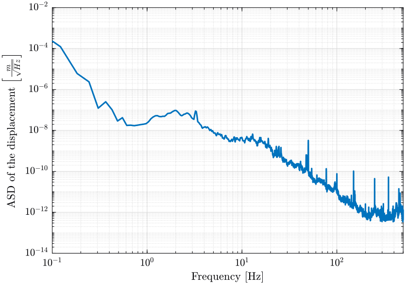
Figure 8: Amplitude Spectral Density of the Displacement

And we also plot the PSD of the displacement in $\frac{{μ u}^{2}}{H z}$ as it is a usual unit used (figure 9). One can then compare this curve with the figure 1.

Copy
figure;
hold on;
plot(f, psd_gm.*1e12);
hold off;
set(gca, 'xscale', 'log');
set(gca, 'yscale', 'log');
xlabel('Frequency [Hz]'); ylabel('PSD of the measured displacement $\left[\frac{{ \mu m }^2}{Hz}\right]$')
xlim([0.1, 500]); ylim([1e-13, 1e3]);

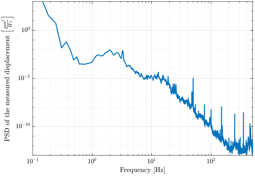
Figure 9: Power Spectral Density of the measured displacement

2.7 Save

We save the PSD of the ground motion for further analysis.

Copy
save('./mat/psd_gm.mat', 'f', 'psd_gm', 'psd_gv');

2.8 Comparison with other measurements of ground motion

Now we will compare with other measurements.

2.8.1 Load the measurement data

First we load the measurement data. Here we have one measurement of the floor motion made at the ESRF in 2018, and one measurement made at CERN.

Copy
id09 = load('./mat/id09_floor_september2018.mat');
cern = load('./mat/ground_motion_dist.mat');

2.8.2 Compute PSD of the measurements

We compute the Power Spectral Densities of the measurements.

Copy
Fs_id09 = 1/(id09.time3(2)-id09.time3(1));
win_id09 = hanning(ceil(10*Fs_id09));
[id09_pxx, id09_f] = pwelch(1e-6*id09.x_y_z(:, 3), win_id09, [], [], Fs_id09);

Copy
Fs_cern = 1/(cern.gm.time(2)-cern.gm.time(1));
win_cern = hanning(ceil(10*Fs_cern));
[cern_pxx, cern_f] = pwelch(cern.gm.signal, win_cern, [], [], Fs_cern);

2.8.3 Compare PSD of Cern, ID09 and ID31

And we compare all the measurements (figure 10).

Copy
figure;
hold on;
plot(id09_f, id09_pxx, 'DisplayName', 'ID09');
plot(cern_f, cern_pxx, 'DisplayName', 'CERN');
plot(f, psd_gm, 'k', 'DisplayName', 'ID31');
hold off;
set(gca, 'XScale', 'log'); set(gca, 'YScale', 'log');
xlabel('Frequency [Hz]'); ylabel('PSD [$m^2/Hz$]');
legend('Location', 'northeast');
xlim([0.1, 500]);

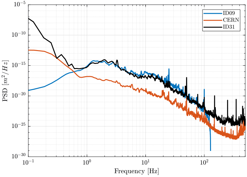
Figure 10: Comparison of the PSD of the ground motion measured at different location