Sercalo Test Bench
Table of Contents
- 1. Introduction
- 2. Identification of the system dynamics
- 3. Huddle Test
- 4. Budget Error
- 4.1. Effect of the Sercalo angle error on the measured distance by the Attocube
- 4.2. Unwanted motion of Sercalo/Newport mirrors perpendicular to its surface
- 4.3. Change in refractive index of the air in the beam path
- 4.4. Thermal Expansion of the Metrology Frame
- 4.5. Estimation of the Sercalo angle error due to Noise
- 5. Plant Uncertainty
- 6. Plant Scaling
- 7. Plant Analysis
- 8. Active Damping
- 9. Decentralized Control of the Sercalo
- 10. Newport Control
- 11. Measurement of the non-repeatability
This report is also available as a pdf.
1 Introduction
1.1 Block Diagram
The block diagram of the setup to be controlled is shown in Fig. 1.
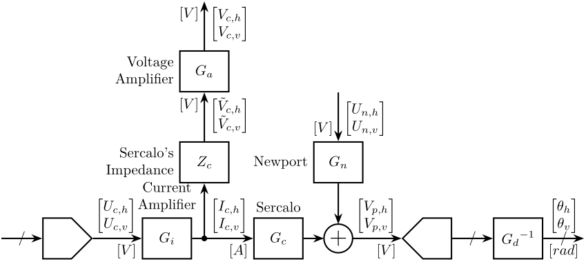
Figure 1: Block Diagram of the Experimental Setup
The transfer functions in the system are:
- Current Amplifier: from the voltage set by the DAC to the current going to the Sercalo’s inductors \[ G_i = \begin{bmatrix} G_{i,h} & 0 \\ 0 & G_{i,v} \end{bmatrix} \text{ in } \left[ \frac{A}{V} \right] \] \[ \begin{bmatrix} I_{c,h} \\ I_{c,v} \end{bmatrix} = G_i \begin{bmatrix} U_{c,h} \\ U_{c,v} \end{bmatrix} \]
- Impedance of the Sercalo that converts the current going to the sercalo to the voltage across the sercalo: \[ Z_c = \begin{bmatrix} Z_{c,h} & 0 \\ 0 & Z_{c,v} \end{bmatrix} \text{ in } \left[ \frac{V}{A} \right] \] \[ \begin{bmatrix} \tilde{V}_{c,h} \\ \tilde{V}_{c,v} \end{bmatrix} = Z_c \begin{bmatrix} I_{c,h} \\ I_{c,v} \end{bmatrix} \]
- Voltage Amplifier: from the voltage across the Sercalo inductors to the measured voltage \[ G_a = \begin{bmatrix} G_{a,h} & 0 \\ 0 & G_{a,v} \end{bmatrix} \text{ in } \left[ \frac{V}{V} \right] \] \[ \begin{bmatrix} V_{c,h} \\ V_{c,v} \end{bmatrix} = G_a \begin{bmatrix} \tilde{V}_{c,h} \\ \tilde{V}_{c,v} \end{bmatrix} \]
- Sercalo: Transfer function from the current going through the sercalo inductors to the 4 quadrant measurement \[ G_c = \begin{bmatrix} G_{\frac{V_{p,h}}{\tilde{U}_{c,h}}} & G_{\frac{V_{p,h}}{\tilde{U}_{c,v}}} \\ G_{\frac{V_{p,v}}{\tilde{U}_{c,h}}} & G_{\frac{V_{p,v}}{\tilde{U}_{c,v}}} \end{bmatrix} \text{ in } \left[ \frac{V}{A} \right] \] \[ \begin{bmatrix} V_{p,h} \\ V_{p,v} \end{bmatrix} = G_c \begin{bmatrix} I_{c,h} \\ I_{c,v} \end{bmatrix} \]
- Newport Transfer function from the command signal of the Newport to the 4 quadrant measurement \[ G_n = \begin{bmatrix} G_{\frac{V_{p,h}}{U_{n,h}}} & G_{\frac{V_{p,h}}{U_{n,v}}} \\ G_{\frac{V_{p,v}}{U_{n,h}}} & G_{\frac{V_{n,v}}{U_{n,v}}} \end{bmatrix} \text{ in } \left[ \frac{V}{V} \right] \] \[ \begin{bmatrix} V_{p,h} \\ V_{p,v} \end{bmatrix} = G_c \begin{bmatrix} V_{n,h} \\ V_{n,v} \end{bmatrix} \]
- 4 Quadrant Diode: the gain of the 4 quadrant diode in [V/rad] is inverse in order to obtain the physical angle of the beam \[ G_d = \begin{bmatrix} G_{d,h} & 0 \\ 0 & G_{d,v} \end{bmatrix} \text{ in } \left[\frac{V}{rad}\right] \]
The block diagram with each transfer function is shown in Fig. 2.
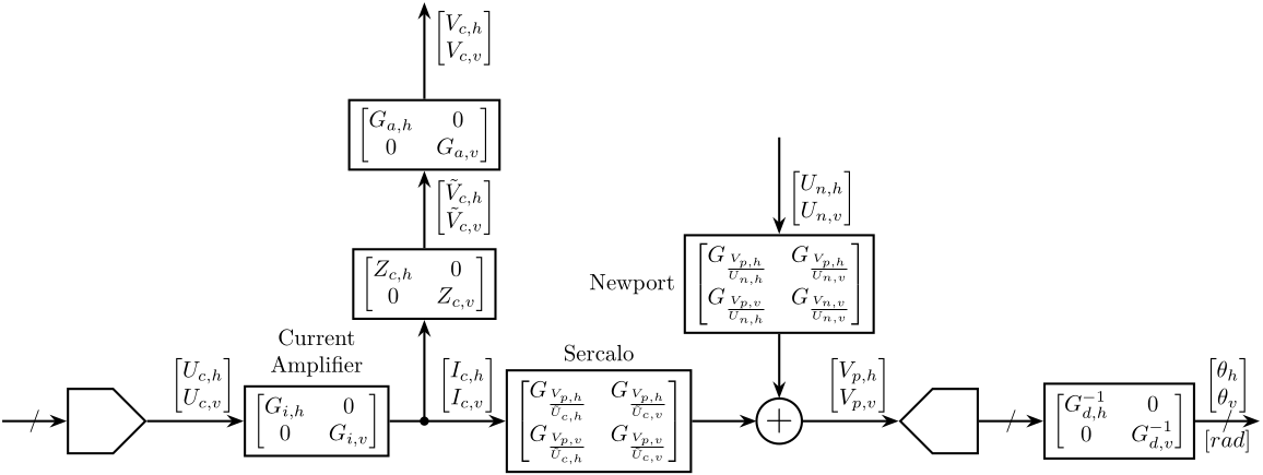
Figure 2: Block Diagram of the Experimental Setup with detailed dynamics
1.2 Sercalo
From the Sercalo documentation, we have the parameters shown on table 1.
| Max. Stroke | Res. Freq. | DC Gain | Gain at res. | RC Res. | |
|---|---|---|---|---|---|
| [deg] | [Hz] | [mA/deg] | [deg/V] | [Ohm] | |
| AX1 (Horizontal) | 5 | 411.13 | 28.4 | 382.9 | 9.41 |
| AX2 (Vertical) | 5 | 252.5 | 35.2 | 350.4 |
The Inductance and DC resistance of the two axis of the Sercalo have been measured:
- \(L_{c,h} = 0.1\ \text{mH}\)
- \(L_{c,v} = 0.1\ \text{mH}\)
- \(R_{c,h} = 9.3\ \Omega\)
- \(R_{c,v} = 8.3\ \Omega\)
Let’s first consider the horizontal direction and we try to model the Sercalo by a spring/mass/damper system (Fig. 3).
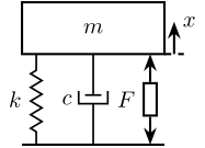
Figure 3: 1 degree-of-freedom model of the Sercalo
The equation of motion is:
\begin{align*} \frac{x}{F} &= \frac{1}{k + c s + m s^2} \\ &= \frac{G_0}{1 + 2 \xi \frac{s}{\omega_0} + \frac{s^2}{\omega_0^2}} \end{align*}with:
- \(G_0 = 1/k\) is the gain at DC in rad/N
- \(\xi = \frac{c}{2 \sqrt{km}}\) is the damping ratio of the system
- \(\omega_0 = \sqrt{\frac{k}{m}}\) is the resonance frequency in rad
The force \(F\) applied to the mass is proportional to the current \(I\) flowing through the voice coils: \[ \frac{F}{I} = \alpha \] with \(\alpha\) is in \(N/A\) and is to be determined.
The current \(I\) is also proportional to the voltage at the output of the buffer:
\begin{align*} \frac{I_c}{U_c} &= \frac{1}{(R + R_c) + L_c s} \\ &\approx 0.02 \left[ \frac{A}{V} \right] \end{align*}Let’s try to determine the equivalent mass and spring values. From table 1, for the horizontal direction: \[ \left| \frac{x}{I} \right|(0) = \left| \alpha \frac{x}{F} \right|(0) = 28.4\ \frac{mA}{deg} = 1.63\ \frac{A}{rad} \]
So: \[ \alpha \frac{1}{k} = 1.63 \Longleftrightarrow k = \frac{\alpha}{1.63} \left[\frac{N}{rad}\right] \]
We also know the resonance frequency: \[ \omega_0 = 411.1\ \text{Hz} = 2583\ \frac{rad}{s} \]
And the gain at resonance:
\begin{align*} \left| \frac{x}{U_c} \right|(j\omega_0) &= \left| 0.02 \frac{x}{I_c} \right| (j\omega_0) \\ &= \left| 0.02 \alpha \frac{x}{F} \right| (j\omega_0) \\ &= 0.02 \alpha \frac{1/k}{2\xi} \\ &= 282.9\ \left[\frac{deg}{V}\right] \\ &= 4.938\ \left[\frac{rad}{V}\right] \end{align*}Thus:
\begin{align*} & \frac{\alpha}{2 \xi k} = 245 \\ \Leftrightarrow & \frac{1.63}{2 \xi} = 245 \\ \Leftrightarrow & \xi = 0.0033 \\ \Leftrightarrow & \xi = 0.33 \% \end{align*}and in terms of the physical properties:
\begin{align*} k &= \frac{\alpha}{1.63}\ \frac{N}{rad} \\ \xi &= 0.0033 \\ m &= \frac{\alpha}{1.1 \cdot 10^7}\ \frac{kg}{m^2} \end{align*}Thus, we have to determine \(\alpha\). This can be done experimentally by determining the gain at DC or at resonance of the system. For that, we need to know the angle of the mirror, thus we need to calibrate the photo-diodes. This will be done using the Newport.
1.3 Optical Setup
1.4 Newport
Parameters of the Newport are shown in Fig. 4.
It’s dynamics for small angle excitation is shown in Fig. 5.
And we have:
\begin{align*} G_{n, h}(0) &= 2.62 \cdot 10^{-3}\ \frac{rad}{V} \\ G_{n, v}(0) &= 2.62 \cdot 10^{-3}\ \frac{rad}{V} \end{align*}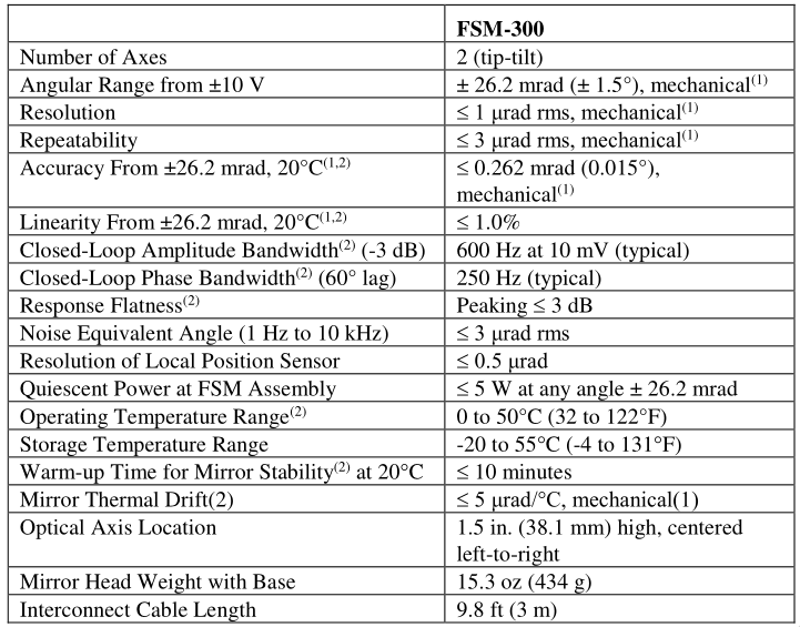
Figure 4: Documentation of the Newport
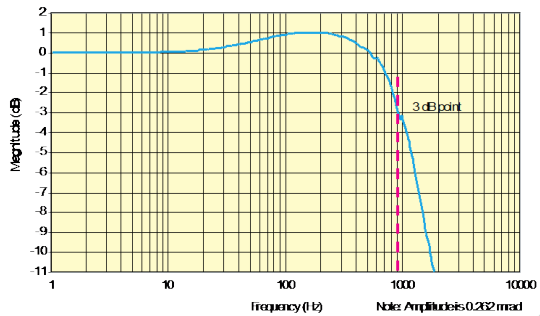
Figure 5: Transfer function of the Newport
1.5 4 quadrant Diode


1.6 ADC/DAC
Let’s compute the theoretical noise of the ADC/DAC.
\begin{align*} \Delta V &= 20 V \\ n &= 16bits \\ q &= \Delta V/2^n = 305 \mu V \\ f_N &= 10kHz \\ \Gamma_n &= \frac{q^2}{12 f_N} = 7.76 \cdot 10^{-13} \frac{V^2}{Hz} \end{align*}with \(\Delta V\) the total range of the ADC, \(n\) its number of bits, \(q\) the quantization, \(f_N\) the sampling frequency and \(\Gamma_n\) its theoretical Power Spectral Density.
2 Identification of the system dynamics
In this section, we seek to identify all the blocks as shown in Fig. 1.
| Signal | Name | Unit |
|---|---|---|
| Voltage Sent to Sercalo - Horizontal | Uch |
[V] |
| Voltage Sent to Sercalo - Vertical | Ucv |
[V] |
| Voltage Sent to Newport - Horizontal | Unh |
[V] |
| Voltage Sent to Newport - Vertical | Unv |
[V] |
| 4Q Photodiode Measurement - Horizontal | Vph |
[V] |
| 4Q Photodiode Measurement - Vertical | Vpv |
[V] |
| Measured Voltage across the Inductance - Horizontal | Vch |
[V] |
| Measured Voltage across the Inductance - Vertical | Vcv |
[V] |
| Newport Metrology - Horizontal | Vnh |
[V] |
| Newport Metrology - Vertical | Vnv |
[V] |
| Attocube Measurement | Va |
[m] |
2.1 Calibration of the 4 Quadrant Diode
Prior to any dynamic identification, we would like to be able to determine the meaning of the 4 quadrant diode measurement. For instance, instead of obtaining transfer function in [V/V] from the input of the sercalo to the measurement voltage of the 4QD, we would like to obtain the transfer function in [rad/V]. This will give insight to physical interpretation.
To calibrate the 4 quadrant photo-diode, we can use the metrology included in the Newport. We can choose precisely the angle of the Newport mirror and see what is the value measured by the 4 Quadrant Diode. We then should be able to obtain the “gain” of the 4QD in [V/rad].
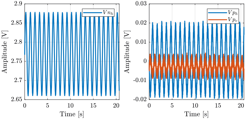
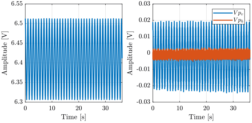
2.1.1 Input / Output data
The identification data is loaded
uh = load('mat/data_cal_pd_h.mat', 't', 'Vph', 'Vpv', 'Vnh');
uv = load('mat/data_cal_pd_v.mat', 't', 'Vph', 'Vpv', 'Vnv');
We remove the first seconds where the Sercalo is turned on.
t0 = 1;

uh.Vph(uh.t<t0) = [];
uh.Vpv(uh.t<t0) = [];
uh.Vnh(uh.t<t0) = [];
uh.t(uh.t<t0)   = [];
uh.t = uh.t - uh.t(1); % We start at t=0

t0 = 1;

uv.Vph(uv.t<t0) = [];
uv.Vpv(uv.t<t0) = [];
uv.Vnv(uv.t<t0) = [];
uv.t(uv.t<t0) = [];
uv.t = uv.t - uv.t(1); % We start at t=0
2.1.2 Linear Regression to obtain the gain of the 4QD
We plot the angle of mirror
Gain of the Newport metrology in [rad/V].
gn0 = 2.62e-3;
The angular displacement of the beam is twice the angular displacement of the Newport mirror.
We do a linear regression \[ y = a x + b \] where:
- \(y\) is the measured voltage of the 4QD in [V]
- \(x\) is the beam angle (twice the mirror angle) in [rad]
- \(a\) is the identified gain of the 4QD in [rad/V]
The linear regression is shown in Fig. 10.
bh = [ones(size(uh.Vnh)) 2*gn0*uh.Vnh]\uh.Vph;
bv = [ones(size(uv.Vnv)) 2*gn0*uv.Vnv]\uv.Vpv;
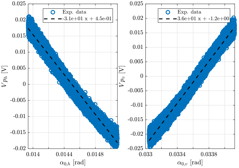
Thus, we obtain the “gain of the 4 quadrant photo-diode as shown on table 2.
| Horizontal [V/rad] | Vertical [V/rad] |
|---|---|
| -31.0 | 36.3 |
Gd = tf([bh(2) 0 ;
         0     bv(2)]);
We obtain:
\begin{align*} \frac{V_{qd,h}}{\alpha_{0,h}} &\approx 0.032\ \left[ \frac{rad}{V} \right] \\ &\approx 32.3\ \left[ \frac{\mu rad}{mV} \right] \end{align*} \begin{align*} \frac{V_{qd,v}}{\alpha_{0,v}} &\approx 0.028\ \left[ \frac{rad}{V} \right] \\ &\approx 27.6\ \left[ \frac{\mu rad}{mV} \right] \end{align*}2.2 Identification of the Sercalo Impedance, Current Amplifier and Voltage Amplifier dynamics
We wish here to determine \(G_i\) and \(G_a\) shown in Fig. 1.
We ignore the electro-mechanical coupling.
2.2.1 Electrical Schematic
The schematic of the electrical circuit used to drive the Sercalo is shown in Fig. 11.

Figure 11: Current Amplifier Schematic
The elements are:
- \(U_c\): the voltage generated by the DAC
- BUF: is a unity-gain open-loop buffer that allows to increase the output current
- \(R\): a chosen resistor that will determine the gain of the current amplifier
- \(L_c\): inductor present in the Sercalo
- \(R_c\): resistance of the inductor
- \(\tilde{V}_c\): voltage measured across the Sercalo’s inductor
- \(V_c\): amplified voltage measured across the Sercalo’s inductor
- \(I_c\) is the current going through the Sercalo’s inductor
The values of the components have been measured for the horizontal and vertical directions:
- \(R_h = 41 \Omega\)
- \(L_{c,h} = 0.1 mH\)
- \(R_{c,h} = 9.3 \Omega\)
- \(R_v = 41 \Omega\)
- \(L_{c,v} = 0.1 mH\)
- \(R_{c,v} = 8.3 \Omega\)
Let’s first determine the transfer function from \(U_c\) to \(I_c\).
We have that: \[ U_c = (R + R_c) I_c + L_c s I_c \]
Thus:
\begin{align} G_i(s) &= \frac{I_c}{U_c} \\ &= \frac{1}{(R + R_c) + L_c s} \\ &= \frac{G_{i,0}}{1 + s/\omega_0} \end{align}with
- \(G_{i,0} = \frac{1}{R + R_c}\)
- \(\omega_0 = \frac{R + R_c}{L_c}\)
Now, determine the transfer function from \(I_c\) to \(\tilde{V}_c\): \[ \tilde{V}_C = R_c I_c + L_c s I_c \] Thus:
\begin{align} Z_c(s) &= \frac{\tilde{V}_c}{I_c} \\ &= R_c + L_c s \end{align}Finally, the transfer function of the voltage amplifier \(G_a\) is simply a low pass filter:
\begin{align} G_a(s) &= \frac{V_c}{\tilde{V}_c} \\ &= \frac{G_{a,0}}{1 + s/\omega_c} \end{align}with
- \(G_{a,0}\) is the gain 1000 (60dB)
- \(\omega_c\) is the cut-off frequency of the voltage amplifier set to 1000Hz
2.2.2 Theoretical Transfer Functions
The values of the components in the current amplifier have been measured.
Rh = 41; % [Ohm]
Lch = 0.1e-3; % [H]
Rch = 9.3; % [Ohm]

Rv = 41; % [Ohm]
Lcv = 0.1e-3; % [H]
Rcv = 8.3; % [Ohm]
Gi = blkdiag(1/(Rh + Rch + Lch * s), 1/(Rv + Rcv + Lcv * s));
Zc = blkdiag(Rch+Lch*s, Rcv+Lcv*s);
Ga = blkdiag(1000/(1 + s/2/pi/1000), 1000/(1 + s/2/pi/1000));

Over the frequency band of interest, the current amplifier transfer function \(G_i\) can be considered as constant. This is the same for the impedance \(Z_c\).
Gi = tf(blkdiag(1/(Rh + Rch), 1/(Rv + Rcv)));
Zc = tf(blkdiag(Rch, Rcv));
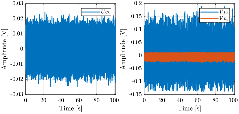
2.2.3 Identified Transfer Functions
Noise is generated using the DAC (\([U_{c,h}\ U_{c,v}]\)) and we measure the output of the voltage amplifier \([V_{c,h}, V_{c,v}]\). From that, we should be able to identify \(G_a Z_c G_i\).
The identification data is loaded.
uh = load('mat/data_uch.mat', 't', 'Uch', 'Vch');
uv = load('mat/data_ucv.mat', 't', 'Ucv', 'Vcv');
We remove the first seconds where the Sercalo is turned on.
win = hanning(ceil(1*fs));
[GaZcGi_h, f] = tfestimate(uh.Uch, uh.Vch, win, [], [], fs);
[GaZcGi_v, ~] = tfestimate(uv.Ucv, uv.Vcv, win, [], [], fs);
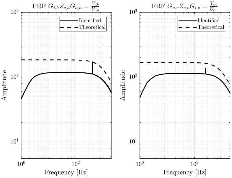
There is a gain mismatch, that is probably due to bad identification of the inductance and resistance measurement of the sercalo inductors. Thus, we suppose \(G_a\) is perfectly known (the gain and cut-off frequency of the voltage amplifier is very accurate) and that \(G_i\) is also well determined as it mainly depends on the resistor used in the amplifier that is well measured.
Gi_resp_h = abs(GaZcGi_h)./squeeze(abs(freqresp(Ga(1,1)*Zc(1,1), f, 'Hz')));
Gi_resp_v = abs(GaZcGi_v)./squeeze(abs(freqresp(Ga(2,2)*Zc(2,2), f, 'Hz')));
Gi = tf(blkdiag(mean(Gi_resp_h(f>20 & f<200)), mean(Gi_resp_v(f>20 & f<200))));
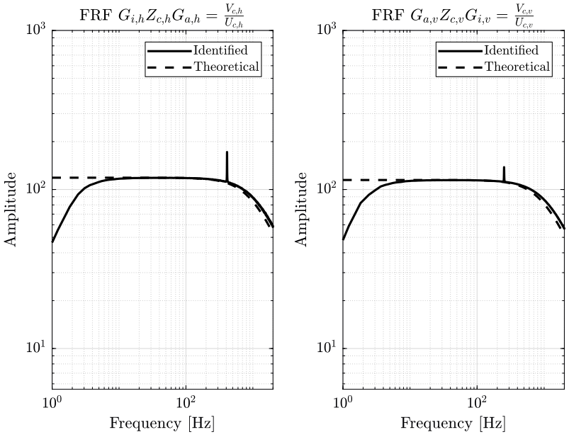
Finally, we have the following transfer functions:
ans = filepath;
if ischar(ans), fid = fopen('/tmp/babel-ZKMGJu/matlab-FA7h5L', 'w'); fprintf(fid, '%s\n', ans); fclose(fid);
else, dlmwrite('/tmp/babel-ZKMGJu/matlab-FA7h5L', ans, '\t')
end
'org_babel_eoe'
Gi,Zc,Ga
'org_babel_eoe'
ans = filepath;
if ischar(ans), fid = fopen('/tmp/babel-ZKMGJu/matlab-FA7h5L', 'w'); fprintf(fid, '%s\n', ans); fclose(fid);
else, dlmwrite('/tmp/babel-ZKMGJu/matlab-FA7h5L', ans, '\t')
end
'org_babel_eoe'
ans =
    'org_babel_eoe'
Gi,Zc,Ga

Gi =

  From input 1 to output...
   1:  0.01275

   2:  0

  From input 2 to output...
   1:  0

   2:  0.01382

Static gain.


Zc =

  From input 1 to output...
   1:  9.3

   2:  0

  From input 2 to output...
   1:  0

   2:  8.3

Static gain.


Ga =

  From input 1 to output...
       6.2832e+06
   1:  ----------
        (s+6283)

   2:  0

  From input 2 to output...
   1:  0

       6.2832e+06
   2:  ----------
        (s+6283)

Continuous-time zero/pole/gain model.
2.3 Identification of the Sercalo Dynamics
We now wish to identify the dynamics of the Sercalo identified by \(G_c\) on the block diagram in Fig. 1.
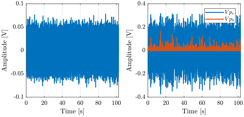
To do so, we inject some noise at the input of the current amplifier \([U_{c,h},\ U_{c,v}]\) (one input after the other) and we measure simultaneously the output of the 4QD \([V_{p,h},\ V_{p,v}]\).
The transfer function obtained will be \(G_c G_i\), and because we have already identified \(G_i\), we can obtain \(G_c\) by multiplying the obtained transfer function matrix by \({G_i}^{-1}\).
2.3.1 Input / Output data
The identification data is loaded
uh = load('mat/data_uch.mat', 't', 'Uch', 'Vph', 'Vpv');
uv = load('mat/data_ucv.mat', 't', 'Ucv', 'Vph', 'Vpv');
We remove the first seconds where the Sercalo is turned on.
t0 = 1;

uh.Uch(uh.t<t0) = [];
uh.Vph(uh.t<t0) = [];
uh.Vpv(uh.t<t0) = [];
uh.t(uh.t<t0)   = [];
uh.t = uh.t - uh.t(1); % We start at t=0

t0 = 1;

uv.Ucv(uv.t<t0) = [];
uv.Vph(uv.t<t0) = [];
uv.Vpv(uv.t<t0) = [];
uv.t(uv.t<t0)   = [];

uv.t = uv.t - uv.t(1); % We start at t=0
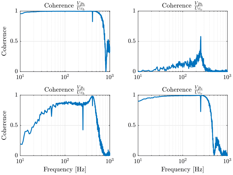
2.3.2 Coherence
The window used for the spectral analysis is an hanning windows with temporal size equal to 1 second.
win = hanning(ceil(1*fs));
[coh_Uch_Vph, f] = mscohere(uh.Uch, uh.Vph, win, [], [], fs);
[coh_Uch_Vpv, ~] = mscohere(uh.Uch, uh.Vpv, win, [], [], fs);
[coh_Ucv_Vph, ~] = mscohere(uv.Ucv, uv.Vph, win, [], [], fs);
[coh_Ucv_Vpv, ~] = mscohere(uv.Ucv, uv.Vpv, win, [], [], fs);
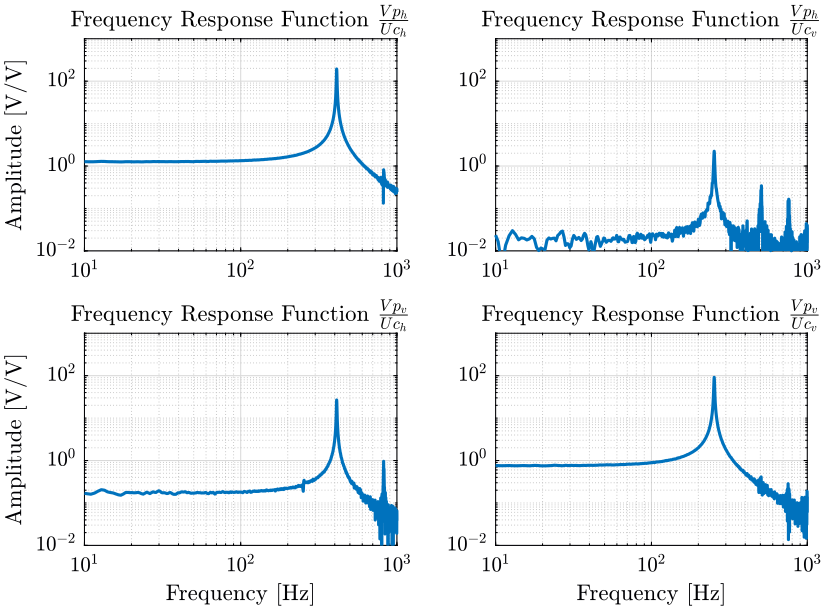
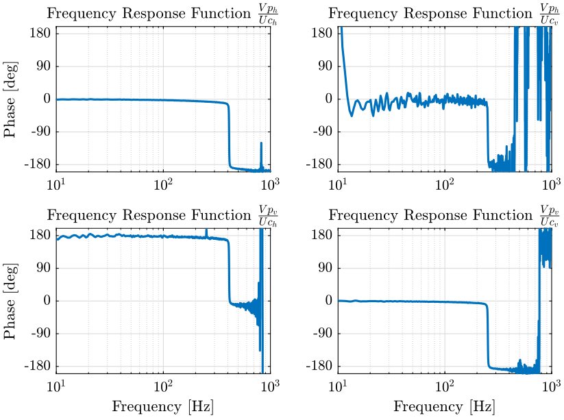
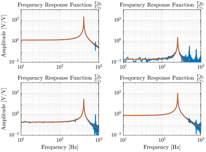
2.3.3 Estimation of the Frequency Response Function Matrix
We compute an estimate of the transfer functions.
[tf_Uch_Vph, f] = tfestimate(uh.Uch, uh.Vph, win, [], [], fs);
[tf_Uch_Vpv, ~] = tfestimate(uh.Uch, uh.Vpv, win, [], [], fs);
[tf_Ucv_Vph, ~] = tfestimate(uv.Ucv, uv.Vph, win, [], [], fs);
[tf_Ucv_Vpv, ~] = tfestimate(uv.Ucv, uv.Vpv, win, [], [], fs);
2.3.4 Time Delay
Now, we would like to remove the time delay included in the FRF prior to the model extraction.
Estimation of the time delay:
Ts_delay = Ts; % [s]

G_delay = tf(1, 1, 'InputDelay', Ts_delay);

G_delay_resp = squeeze(freqresp(G_delay, f, 'Hz'));
We then remove the time delay from the frequency response function.
tf_Uch_Vph = tf_Uch_Vph./G_delay_resp;
tf_Uch_Vpv = tf_Uch_Vpv./G_delay_resp;
tf_Ucv_Vph = tf_Ucv_Vph./G_delay_resp;
tf_Ucv_Vpv = tf_Ucv_Vpv./G_delay_resp;
2.3.5 Extraction of a transfer function matrix
First we define the initial guess for the resonance frequencies and the weights associated.
freqs_res_uh = [410]; % [Hz]
freqs_res_uv = [250]; % [Hz]
We then make an initial guess on the complex values of the poles.
xi = 0.001; % Approximate modal damping
poles_uh = [2*pi*freqs_res_uh*(xi + 1i), 2*pi*freqs_res_uh*(xi - 1i)];
poles_uv = [2*pi*freqs_res_uv*(xi + 1i), 2*pi*freqs_res_uv*(xi - 1i)];
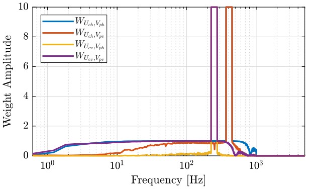
We then define the weight that will be used for the fitting. Basically, we want more weight around the resonance and at low frequency (below the first resonance). Also, we want more importance where we have a better coherence. Finally, we ignore data above some frequency.
weight_Uch_Vph = coh_Uch_Vph';
weight_Uch_Vpv = coh_Uch_Vpv';
weight_Ucv_Vph = coh_Ucv_Vph';
weight_Ucv_Vpv = coh_Ucv_Vpv';

alpha = 0.1;

for freq_i = 1:length(freqs_res_uh)
  weight_Uch_Vph(f>(1-alpha)*freqs_res_uh(freq_i) & f<(1 + alpha)*freqs_res_uh(freq_i)) = 10;
  weight_Uch_Vpv(f>(1-alpha)*freqs_res_uh(freq_i) & f<(1 + alpha)*freqs_res_uh(freq_i)) = 10;
  weight_Ucv_Vph(f>(1-alpha)*freqs_res_uv(freq_i) & f<(1 + alpha)*freqs_res_uv(freq_i)) = 10;
  weight_Ucv_Vpv(f>(1-alpha)*freqs_res_uv(freq_i) & f<(1 + alpha)*freqs_res_uv(freq_i)) = 10;
end

weight_Uch_Vph(f>1000) = 0;
weight_Uch_Vpv(f>1000) = 0;
weight_Ucv_Vph(f>1000) = 0;
weight_Ucv_Vpv(f>1000) = 0;
The weights are shown in Fig. 20.
When we set some options for vfit3.
opts = struct();

opts.stable = 1;    % Enforce stable poles
opts.asymp = 1;     % Force D matrix to be null
opts.relax = 1;     % Use vector fitting with relaxed non-triviality constraint
opts.skip_pole = 0; % Do NOT skip pole identification
opts.skip_res = 0;  % Do NOT skip identification of residues (C,D,E)
opts.cmplx_ss = 0;  % Create real state space model with block diagonal A

opts.spy1 = 0;      % No plotting for first stage of vector fitting
opts.spy2 = 0;      % Create magnitude plot for fitting of f(s)
We define the number of iteration.
Niter = 5;
An we run the vectfit3 algorithm.
for iter = 1:Niter
  [SER_Uch_Vph, poles, ~, fit_Uch_Vph] = vectfit3(tf_Uch_Vph.', 1i*2*pi*f, poles_uh, weight_Uch_Vph, opts);
end
for iter = 1:Niter
  [SER_Uch_Vpv, poles, ~, fit_Uch_Vpv] = vectfit3(tf_Uch_Vpv.', 1i*2*pi*f, poles_uh, weight_Uch_Vpv, opts);
end
for iter = 1:Niter
  [SER_Ucv_Vph, poles, ~, fit_Ucv_Vph] = vectfit3(tf_Ucv_Vph.', 1i*2*pi*f, poles_uv, weight_Ucv_Vph, opts);
end
for iter = 1:Niter
  [SER_Ucv_Vpv, poles, ~, fit_Ucv_Vpv] = vectfit3(tf_Ucv_Vpv.', 1i*2*pi*f, poles_uv, weight_Ucv_Vpv, opts);
end

And finally, we create the identified \(G_c\) matrix by multiplying by \({G_i}^{-1}\).
G_Uch_Vph = tf(minreal(ss(full(SER_Uch_Vph.A),SER_Uch_Vph.B,SER_Uch_Vph.C,SER_Uch_Vph.D)));
G_Ucv_Vph = tf(minreal(ss(full(SER_Ucv_Vph.A),SER_Ucv_Vph.B,SER_Ucv_Vph.C,SER_Ucv_Vph.D)));
G_Uch_Vpv = tf(minreal(ss(full(SER_Uch_Vpv.A),SER_Uch_Vpv.B,SER_Uch_Vpv.C,SER_Uch_Vpv.D)));
G_Ucv_Vpv = tf(minreal(ss(full(SER_Ucv_Vpv.A),SER_Ucv_Vpv.B,SER_Ucv_Vpv.C,SER_Ucv_Vpv.D)));

Gc = [G_Uch_Vph, G_Ucv_Vph;
      G_Uch_Vpv, G_Ucv_Vpv]*inv(Gi);
2.4 Identification of the Newport Dynamics
We here identify the transfer function from a reference sent to the Newport \([U_{n,h},\ U_{n,v}]\) to the measurement made by the 4QD \([V_{p,h},\ V_{p,v}]\).
To do so, we inject noise to the Newport \([U_{n,h},\ U_{n,v}]\) and we record the 4QD measurement \([V_{p,h},\ V_{p,v}]\).
2.4.1 Input / Output data
The identification data is loaded
uh = load('mat/data_unh.mat', 't', 'Unh', 'Vph', 'Vpv');
uv = load('mat/data_unv.mat', 't', 'Unv', 'Vph', 'Vpv');
We remove the first seconds where the Sercalo is turned on.
t0 = 3;

uh.Unh(uh.t<t0) = [];
uh.Vph(uh.t<t0) = [];
uh.Vpv(uh.t<t0) = [];
uh.t(uh.t<t0)   = [];
uh.t = uh.t - uh.t(1); % We start at t=0

t0 = 1.5;

uv.Unv(uv.t<t0) = [];
uv.Vph(uv.t<t0) = [];
uv.Vpv(uv.t<t0) = [];
uv.t(uv.t<t0)   = [];

uv.t = uv.t - uv.t(1); % We start at t=0

2.4.2 Coherence
The window used for the spectral analysis is an hanning windows with temporal size equal to 1 second.
win = hanning(ceil(1*fs));
[coh_Unh_Vph, f] = mscohere(uh.Unh, uh.Vph, win, [], [], fs);
[coh_Unh_Vpv, ~] = mscohere(uh.Unh, uh.Vpv, win, [], [], fs);
[coh_Unv_Vph, ~] = mscohere(uv.Unv, uv.Vph, win, [], [], fs);
[coh_Unv_Vpv, ~] = mscohere(uv.Unv, uv.Vpv, win, [], [], fs);

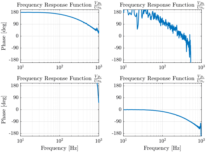
2.4.3 Estimation of the Frequency Response Function Matrix
We compute an estimate of the transfer functions.
[tf_Unh_Vph, f] = tfestimate(uh.Unh, uh.Vph, win, [], [], fs);
[tf_Unh_Vpv, ~] = tfestimate(uh.Unh, uh.Vpv, win, [], [], fs);
[tf_Unv_Vph, ~] = tfestimate(uv.Unv, uv.Vph, win, [], [], fs);
[tf_Unv_Vpv, ~] = tfestimate(uv.Unv, uv.Vpv, win, [], [], fs);

2.4.4 Time Delay
Now, we would like to remove the time delay included in the FRF prior to the model extraction.
Estimation of the time delay:
Ts_delay = 0.0005; % [s]

G_delay = tf(1, 1, 'InputDelay', Ts_delay);

G_delay_resp = squeeze(freqresp(G_delay, f, 'Hz'));
We then remove the time delay from the frequency response function.

2.4.5 Extraction of a transfer function matrix
From Fig. 26, it seems reasonable to model the Newport dynamics as diagonal and constant.
Gn = blkdiag(tf(mean(abs(tf_Unh_Vph(f>10 & f<100)))), tf(mean(abs(tf_Unv_Vpv(f>10 & f<100)))));
2.5 Full System
We now have identified:
- \(G_i\)
- \(G_a\)
- \(G_c\)
- \(G_n\)
- \(G_d\)
We name the input and output of each transfer function:
Gi.InputName = {'Uch', 'Ucv'};
Gi.OutputName = {'Ich', 'Icv'};

Zc.InputName = {'Ich', 'Icv'};
Zc.OutputName = {'Vtch', 'Vtcv'};

Ga.InputName = {'Vtch', 'Vtcv'};
Ga.OutputName = {'Vch', 'Vcv'};

Gc.InputName = {'Ich', 'Icv'};
Gc.OutputName = {'Vpch', 'Vpcv'};

Gn.InputName = {'Unh', 'Unv'};
Gn.OutputName = {'Vpnh', 'Vpnv'};

Gd.InputName = {'Rh', 'Rv'};
Gd.OutputName = {'Vph', 'Vpv'};
Sh = sumblk('Vph = Vpch + Vpnh');
Sv = sumblk('Vpv = Vpcv + Vpnv');
inputs  = {'Uch', 'Ucv', 'Unh', 'Unv'};
outputs = {'Vch', 'Vcv', 'Ich', 'Icv', 'Rh', 'Rv', 'Vph', 'Vpv'};

sys = connect(Gi, Zc, Ga, Gc, Gn, inv(Gd), Sh, Sv, inputs, outputs);
The file mat/plant.mat is accessible here.
save('mat/plant.mat', 'sys', 'Gi', 'Zc', 'Ga', 'Gc', 'Gn', 'Gd');
3 Huddle Test
The goal is to determine the noise of the photodiodes as well as the noise of the Attocube interferometer.
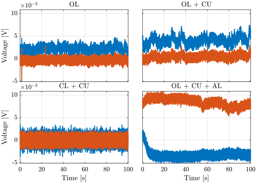
Multiple measurements are done with different experimental configuration as follow:
| Number | OL/CL | Compensation Unit | Aluminum |
|---|---|---|---|
| 1 | Open Loop | ||
| 2 | Open Loop | Compensation Unit | |
| 3 | Closed Loop | Compensation Unit | |
| 4 | Open Loop | Compensation Unit | Aluminum |
| 5 | Closed Loop | Compensation Unit | Aluminum |
3.1 Load Data
ht_1 = load('./mat/data_huddle_test_1.mat', 't', 'Vph', 'Vpv', 'Va');
ht_2 = load('./mat/data_huddle_test_2.mat', 't', 'Vph', 'Vpv', 'Va');
ht_3 = load('./mat/data_huddle_test_3.mat', 't', 'Uch', 'Ucv', 'Vph', 'Vpv', 'Va');
ht_4 = load('./mat/data_huddle_test_4.mat', 't', 'Vph', 'Vpv', 'Va');
% ht_5 = load('./mat/data_huddle_test_5.mat', 't', 'Uch', 'Ucv', 'Vph', 'Vpv', 'Va');
fs = 1e4;
3.2 Pre-processing
t0 = 1; % [s]

tend = 100; % [s]

ht_s = {ht_1 ht_2 ht_3 ht_4}

for i = 1:length(ht_s)
  ht_s{i}.Vph(ht_s{i}.t<t0) = [];
  ht_s{i}.Vpv(ht_s{i}.t<t0) = [];
  ht_s{i}.Va(ht_s{i}.t<t0)  = [];
  ht_s{i}.t(ht_s{i}.t<t0)   = [];

  ht_s{i}.t = ht_s{i}.t - ht_s{i}.t(1); % We start at t=0

  ht_s{i}.Vph(tend*fs+1:end) = [];
  ht_s{i}.Vpv(tend*fs+1:end) = [];
  ht_s{i}.Va(tend*fs+1:end)  = [];
  ht_s{i}.t(tend*fs+1:end)   = [];

  ht_s{i}.Va = ht_s{i}.Va - mean(ht_s{i}.Va);
end

ht_1 = ht_s{1};
ht_2 = ht_s{2};
ht_3 = ht_s{3};
ht_4 = ht_s{4};
3.3 Filter data with low pass filter
We filter the data with a first order low pass filter with a crossover frequency of \(\omega_0\).
w0 = 50; % [Hz]

G_lpf = 1/(1 + s/2/pi/w0);

ht_1.Vaf = lsim(G_lpf, ht_1.Va, ht_1.t);
ht_2.Vaf = lsim(G_lpf, ht_2.Va, ht_2.t);
ht_3.Vaf = lsim(G_lpf, ht_3.Va, ht_3.t);
ht_4.Vaf = lsim(G_lpf, ht_4.Va, ht_4.t);
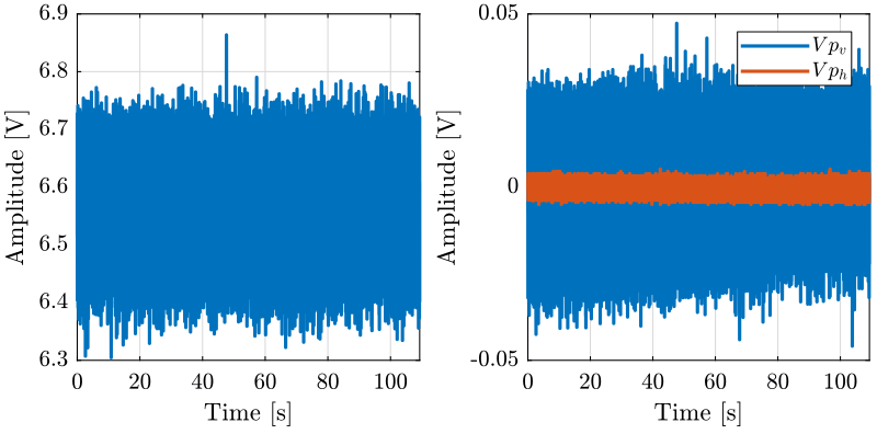
3.4 Time domain plots

3.5 Power Spectral Density
win = hanning(ceil(1*fs));
[psd_Va1, f] = pwelch(ht_1.Va, win, [], [], fs);
[psd_Va2, ~] = pwelch(ht_2.Va, win, [], [], fs);
[psd_Va3, ~] = pwelch(ht_3.Va, win, [], [], fs);
[psd_Va4, ~] = pwelch(ht_4.Va, win, [], [], fs);
[psd_Vph1, ~] = pwelch(ht_1.Vph, win, [], [], fs);
[psd_Vph2, ~] = pwelch(ht_2.Vph, win, [], [], fs);
[psd_Vph3, ~] = pwelch(ht_3.Vph, win, [], [], fs);
[psd_Vph4, ~] = pwelch(ht_4.Vph, win, [], [], fs);
[psd_Vpv1, ~] = pwelch(ht_1.Vpv, win, [], [], fs);
[psd_Vpv2, ~] = pwelch(ht_2.Vpv, win, [], [], fs);
[psd_Vpv3, ~] = pwelch(ht_3.Vpv, win, [], [], fs);
[psd_Vpv4, ~] = pwelch(ht_4.Vpv, win, [], [], fs);
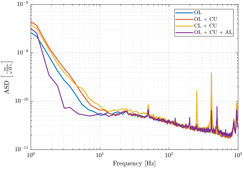
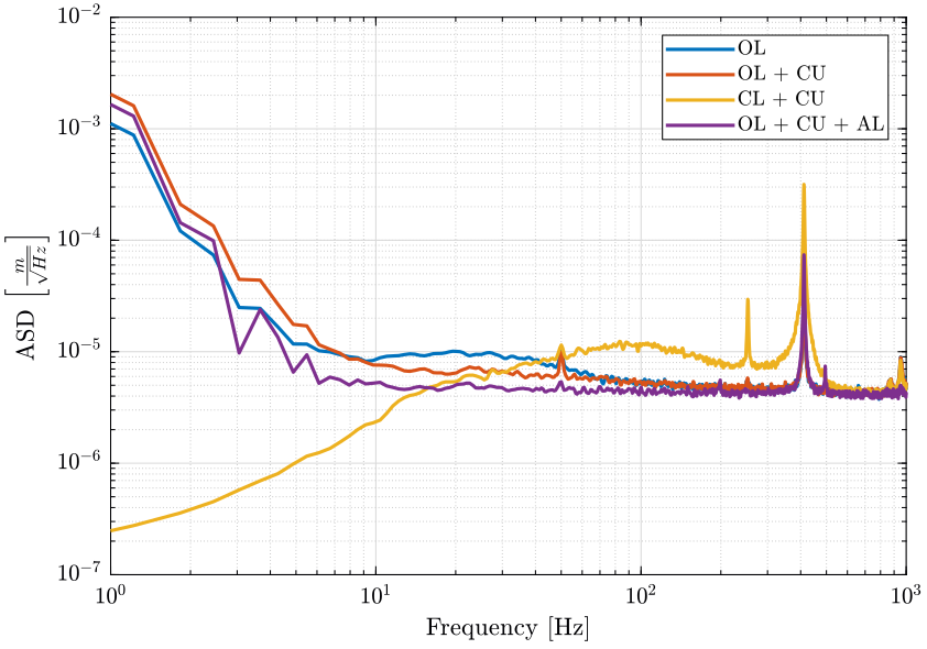
3.6 Conclusion
The Attocube’s “Environmental Compensation Unit” does not have a significant effect on the stability of the measurement.
4 Budget Error
Goals:
- List all sources of error and compute their effects on the Attocube measurement
- Think about how to determine the value of the individual sources of error
- Sum all the sources of error and determine the limiting ones
Sources of error for the Attocube measurement:
- Beam non-perpendicularity to the concave mirror is linked to the non-perfect feedback loop:
- We have only finite gain / limited bandwidth so the Sercalo mirror angle will not be perfect
- The non-perpendicularity is measured by the 4QD and is used as the feedback signal, however this signal is noisy and even with infinite gain, this noise will be transmitted to the angle of the beam
- Sercalo/Newport unwanted translation perpendicular to its surface.
This can be due to:
- Non idealities in the mechanics of the Sercalo
- Temperature variations
- The reproducible part of the perpendicular translation with respect to the angle of the Sercalo can be taken into account and subtracted from the Attocube measurement
- Temperature variations of the metrology frame
- Change in the refractive air index in the beam path. This can be due to change of Temperature, Pressure and Humidity of the air in the beam path
Procedure:
- in section 4.1: We estimate the effect of an angle error of the Sercalo mirror on the Attocube measurement
- in section 4.2: The effect of perpendicular motion of the Newport and Sercalo mirrors on the Attocube measurement is determined.
- in section 4.3: We estimate the expected change of refractive index of the air in the beam path and the resulting Attocube measurement error
- in section 4.5: The feedback system using the 4 quadrant diode and the Sercalo is studied. Sensor noise, actuator noise and their effects on the control error is discussed.
4.1 Effect of the Sercalo angle error on the measured distance by the Attocube
To simplify, we suppose that the Newport mirror is a flat mirror (instead of a concave one).
The geometry of the setup is shown in Fig. 33 where:
- \(O\) is the reference surface of the Attocube
- \(S\) is the point where the beam first hits the Sercalo mirror
- \(X\) is the point where the beam first hits the Newport mirror
- \(\delta \theta_c\) is the angle error from its ideal 45 degrees
We define the angle error range \(\delta \theta_c\) where we want to evaluate the distance error \(\delta L\) measured by the Attocube.
thetas_c = logspace(-7, -4, 100); % [rad]
The geometrical parameters of the setup are defined below.
H = 0.05; % [m]
L = 0.05; % [m]
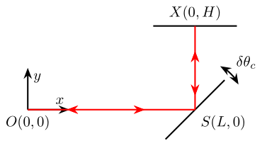
Figure 33: Schematic of the geometry used to evaluate the effect of \(\delta \theta_c\) on the measured distance \(\delta L\)
The nominal points \(O\), \(S\) and \(X\) are defined.
O = [-L, 0];
S = [0, 0];
X = [0, H];
Thus, the initial path length \(L\) is:
path_nominal = norm(S-O) + norm(X-S) + norm(S-X) + norm(O-S);
We now compute the new path length when there is an error angle \(\delta \theta_c\) on the Sercalo mirror angle.
path_length = zeros(size(thetas_c));

for i = 1:length(thetas_c)
    theta_c = thetas_c(i);
    Y = [H*tan(2*theta_c), H];
    M = 2*H/(tan(pi/4-theta_c)+1/tan(2*theta_c))*[1, tan(pi/4-theta_c)];
    T = [-L, M(2)+(L+M(1))*tan(4*theta_c)];

    path_length(i) = norm(S-O) + norm(Y-S) + norm(M-Y) + norm(T-M);
end
We then compute the distance error and we plot it as a function of the Sercalo angle error (Fig. 34).
path_error = path_length - path_nominal;

Figure 34: Effect of an angle error of the Sercalo on the distance error measured by the Attocube (png, pdf)
And we plot the beam path using Matlab for an high angle to verify that the code is working (Fig. 35).
theta = 2*2*pi/360; % [rad]
H = 0.05; % [m]
L = 0.05; % [m]

O = [-L, 0];
S = [0, 0];
X = [0, H];
Y = [H*tan(2*theta), H];
M = 2*H/(tan(pi/4-theta)+1/tan(2*theta))*[1, tan(pi/4-theta)];
T = [-L, M(2)+(L+M(1))*tan(4*theta)];
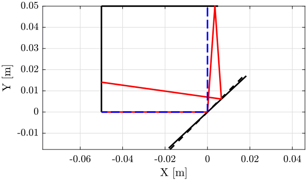
Based on Fig. 34, we see that an angle error \(\delta\theta_c\) of the Sercalo mirror induces a distance error \(\delta L\) measured by the Attocube which is dependent of the square of \(\delta \theta_c\):
\begin{equation} \delta L = \delta\theta_c^2 \end{equation}with:
- \(\delta L\) expressed in [m]
- \(\delta \theta_c\) in [rad]
Some example are shown in table 4.
The tracking error of the feedback system used to position the Sercalo mirror should thus be limited to few micro-meters.
| Angle Error \(\delta \theta_c\) | Distance measurement error \(\delta L\) |
|---|---|
| \(1\,\mu\text{rad}\) | \(1\, nm\) |
| \(5\,\mu\text{rad}\) | \(25\, nm\) |
| \(10\,\mu\text{rad}\) | \(100\, nm\) |
4.2 Unwanted motion of Sercalo/Newport mirrors perpendicular to its surface
From Figs 36 and 37, it is clear that perpendicular motions of the Sercalo mirror and of the Newport mirror have an impact on the measured distance by the Attocube interferometer.
More precisely, if the note:
- \(\delta d_c\) the perpendicular motion of the Sercalo’s mirror
- \(\delta d_n\) the perpendicular motion of the Newport’s mirror
We have that:
\begin{align} \delta L &= 2 \cdot \delta d_c \\ \delta L &= 2 \cdot \delta d_n \end{align}Note here that \(\delta L\) denote the change of beam traveled distance. The error in measured distance by the Attocube will we \(\delta L/2\).
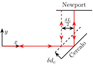
Figure 36: Effect of a Perpendicular motion of the Sercalo Mirror
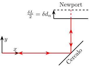
Figure 37: Effect of a Perpendicular motion of the Newport Mirror
The motion of the both Sercalo’s and Newport’s mirrors perpendicular to its surface is fully transmitted to the measured distance by the Attocube interferometer.
This motion can be measured and the repeatable part can be compensated. However, the non repeatability of this motion should be less than few nano-meters.
4.3 Change in refractive index of the air in the beam path
Three physical properties of the air makes change of the Attocube measurement:
- Temperature: \(K_T \approx 1 ppmK^{-1}\)
- Pressure: \(K_P \approx 0.27 ppm hPa^{-1}\)
- Humidity: \(K_{HR} \approx 0.01 ppm \% RH^{-1}\)
These physical properties should change relatively slowly, however, for a beam path of 100mm:
| Air property Variations | Measurement error |
|---|---|
| \(\Delta T = 1^oC\) | 100nm |
| \(\Delta P = 1hPa\) | 27nm |
| \(\Delta 10\%RH\) | 10nm |
An Environmental Compensation Unit is used and can compensate for variations or air properties up to:
| Air property Variations | Measurement error |
|---|---|
| \(\Delta T = \pm 0.1^oC\) | \(\pm 10\,\text{nm}\) |
| \(\Delta P = \pm 1hPa\) | \(\pm 25\,\text{nm}\) |
| \(\Delta \pm 2\%RH\) | \(\pm 2\,\text{nm}\) |
The total measurement error induced by air properties variations is then:
\begin{equation} \sqrt{20^2 + 50^2 + 4^2} = 54nm \end{equation}The beam path should be protected using aluminum to minimize the change in refractive index of the air in the beam path.
4.4 Thermal Expansion of the Metrology Frame
The material used for the metrology frame is Aluminum. Its linear thermal expansion coefficient is \(\alpha = 23 \cdot 10^{-6} K^{-1}\).
The distance between the Attocube head and the Attocube is approximatively equal to 5cm. \[ \frac{\delta L}{\delta T} \approx 0.05 \cdot 23 \cdot 10^{-6} \approx 1\,\frac{\mu m}{{}^oC} \] If invar is used (\(\alpha = 1.2 \cdot 10^{-6} \, K^{-1}\)): \[ \frac{\delta L}{\delta T} \approx 60 \frac{nm}{{}^oC} \]
Thus, the temperature of the metrology frame should be kept constant to less than \(0.1\,^oC\).
4.5 Estimation of the Sercalo angle error due to Noise
In this section, we seek to estimate the angle error \(\delta \theta\)
Consider the block diagram in Fig. 38 with:
- \(G\): represents the transfer function from a voltage applied by the Speedgoat DAC used for the Sercalo to the Beam angle
- \(K\): is the control law used
The signals are:
- \(\delta \theta\): is the “true” laser beam angle
- \(\delta \theta_m\): is the measured beam angle (\(\delta \theta_m = \delta \theta + n_\theta\))
- \(n_\theta\): is the measurement noise of the laser beam angle using the 4 quadrant diode.
It includes:
- ADC noise
- \(1/f\) noise, Shot noise, Ambian noise, Intensity noise…
- \(d_u\): is noise at the input of the Sercalo.
It includes:
- DAC noise of the speadgoat
- \(d\): is disturbance on the angle of the beam.
It includes:
- Angle variations of the Newport mirror
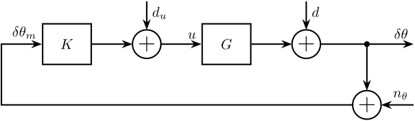
Figure 38: Block Diagram of the Feedback system
4.5.1 Estimation of sources of noise and disturbances
Let’s estimate the values of \(d_u\), \(d\) and \(n_\theta\).
4.5.1.1 ADC Quantization Noise
The ADC quantization noise is:
\begin{equation} \Gamma_\text{ADC} = \frac{\left(\frac{\Delta V}{2^n}\right)^2}{12 f_s} \text{ in } \left[ \frac{V^2}{Hz} \right] \end{equation}with:
- \(\Delta V\): is the range of the ADC in \([V]\)
- \(n\): is the number of ADC’s bits
- \(f_s\): is the sampling frequency in \([Hz]\)
For the ADC used:
- \(\Delta V = 20\, V\)
- \(n = 16\)
- \(f_s = 10\, kHz\)
4.5.1.2 DAC Quantization Noise
The DAC quantization noise is:
\begin{equation} \Gamma_\text{DAC} = \frac{\left(\frac{\Delta V}{2^n}\right)^2}{12 f_s} \text{ in } \left[ \frac{V^2}{Hz} \right] \end{equation}with:
- \(\Delta V\): is the range of the DAC in \([V]\)
- \(n\): is the number of DAC’s bits
- \(f_s\): is the sampling frequency in \([Hz]\)
For the DAC used:
- \(\Delta V = 20\, V\)
- \(n = 16\)
- \(f_s = 10\, kHz\)
4.5.1.3 Noise of the Newport Mirror angle
Plus, we estimate the effect of DAC quantization noise on the angle error on the Newport mirror.
The gain of the Newport is:
\begin{align*} \frac{\theta_n}{V_n} &= \frac{26.2}{10}\ \left[ \frac{mrad}{V} \right] \\ &= 2.62 \cdot 10^{-3}\ \left[ \frac{rad}{V} \right] \end{align*} \begin{align*} \Gamma_{\theta_n}(f) &= \left(\frac{\theta_n}{V_n}\right)^2 \cdot \Gamma_\text{DAC}(f) \\ &= (2.62 \cdot 10^{-3})^2 \cdot 7.76 \cdot 10^{-13} \\ &= 3.96 \cdot 10^{-18}\,\left[ \frac{rad^2}{Hz} \right] \end{align*}If we integrate that to obtain an rms value:
\begin{align*} \theta_{n, rms} &= \sqrt{\int_{-f_s/2}^{f_s/2} \Gamma_{\theta_n}(f) df} \\ &= 0.2\, \mu rad \end{align*}Which is much less than the noise equivalent angle specified by Newport: \(3\, \mu rad\,[rms]\). Thus, quantization error of the DAC is not a problem.
We expect the angle noise of the Newport mirror to be around \(3\, \mu rad\,[rms]\) which is \(6\, \mu rad\,[rms]\) for the beam angle.
If we suppose a white noise, the power spectral density of the beam angle due to the noise of the Newport mirror corresponds to:
\begin{align*} \Gamma_{d} &= \frac{(6 \cdot 10^{-6})^2}{f_s}\ \left[ \frac{rad^2}{Hz} \right] \\ &= 3.6 \cdot 10^{-15}\ \left[ \frac{rad^2}{Hz} \right] \end{align*}4.5.1.4 Disturbances due the Newport Mirror Rotation
We will rotate the Newport mirror in order to simulate a displacement of the Sample:
- The angle range for the Newport mirror is \(\pm 26.2\ mrad = \pm 1.5^o\)
- The radius of the concave mirror is 200 mm
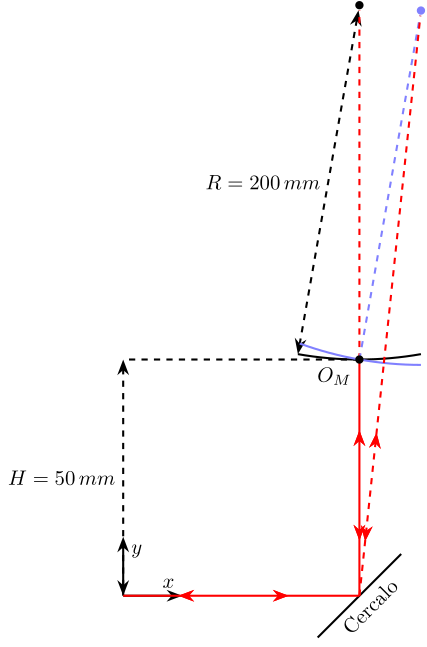
Figure 39: Rotation of the (concave) Newport mirror
If we suppose small angles, the corresponding beam deviation is: \[ \delta \theta \approx 2*\frac{\alpha R}{H + R} = 1.6 \alpha \] where \(\alpha\) is the rotation of the Newport mirror.
4.5.2 Perfect Control
If the feedback is perfect, the Sercalo angle error will be equal to the 4 quadrant diode noise. Let’s estimate the 4QD noise in radians.
If we note \(V_1\), \(V_2\), \(V_3\) and \(V_4\) the voltage of each of the quadrant, a measurement error \(\delta V_i\) of one of the quadrant will have an effect \(\delta \theta\) on the measured angle: \[ \delta\theta = G \frac{\delta V_i}{V_1 + V_2 + V_3 + V_4} \] with \(G\) is the gain of the 4QD in [rad].
We should then have that the voltage of each quadrant is as large as possible. Suppose here that \(V_i \approx 5V\), \(\delta V_i = 1mV\) and \(G = 0.03\,rad\), we obtain: \[ \delta \theta = 0.03 \frac{0.001}{20} = 1.5\, \mu\text{rad} \] This then corresponds to \[ \delta L = 10^{-6} \cdot \delta \theta = 1.5\,nm \]
If we just consider the ADC noise:
- the ADC range is \(\pm 10V\) with \(16\text{ bits}\).
- thus, the LSB corresponds to: \[ \frac{20}{2^{16}} \approx 0.000305\,V = 0.305\,mV \]
- this corresponds to an error \(\delta L \approx 0.5 nm\)
4.5.3 Error due to DAC noise used for the Sercalo
load('./mat/plant.mat', 'Gi', 'Gc', 'Gd');
G = inv(Gd)*Gc*Gi;
Dynamical estimation:
- ASD of DAC noise used for the Sercalo
- Multiply by transfer function from Sercalo voltage to angle estimation using the 4QD
freqs = logspace(1, 3, 1000);

fs = 1e4;

% ASD of the DAC voltage going to the Sercalo in [V/sqrt(Hz)]
asd_uc = (20/2^16)/sqrt(12*fs)*ones(length(freqs), 1);

% ASD of the measured angle by the QD in [rad/sqrt(Hz)]
asd_theta = asd_uc.*abs(squeeze(freqresp(G(1,1), freqs, 'Hz')));

figure;
loglog(freqs, asd_theta)
Then the corresponding ASD of the measured displacement by the interferometer is:
asd_L = asd_theta*10^(-6); % [m/sqrt(Hz)]
And we integrate that to have the RMS value:
cps_L = 1/pi*cumtrapz(2*pi*freqs, (asd_L).^2);
The RMS value is:
sqrt(cps_L(end))
1.647e-11
figure;
loglog(freqs, cps_L)
Let’s estimate the beam angle error corresponding to 1 LSB of the sercalo’s DAC. Gain of the Sercalo is approximatively 5 degrees for 10V. However the beam angle deviation is 4 times the angle deviation of the sercalo mirror, thus:
d_alpha = 4*(20/2^16)*(5*pi/180)/10 % [rad]
1.0653e-05
This corresponds to a measurement error of the Attocube equals to (in [m])
1e-6*d_alpha % [m]
1.0653e-11
The DAC noise use for the Sercalo does not limit the performance of the system.
5 Plant Uncertainty
5.1 Coprime Factorization
load('mat/plant.mat', 'sys', 'Gi', 'Zc', 'Ga', 'Gc', 'Gn', 'Gd');
[fact, Ml, Nl] = lncf(Gc*Gi);
6 Plant Scaling
The goal is the scale the plant prior to control synthesis. This will simplify the choice of weighting functions and will yield useful insight on the controllability of the plant.
| Value | Unit | Variable Name | |
|---|---|---|---|
| Expected perturbations | 1 | [V] | \(U_n\) |
| Maximum input usage | 10 | [V] | \(U_c\) |
| Maximum wanted error | 10 | [\(\mu rad\)] | \(\theta\) |
| Measured noise | 5 | [\(\mu rad\)] |
6.1 Control Objective
The maximum expected stroke is \(y_\text{max} = 3mm \approx 5e^{-2} rad\) at \(1Hz\). The maximum wanted error is \(e_\text{max} = 10 \mu rad\).
Thus, we require the sensitivity function at \(\omega_0 = 1\text{ Hz}\):
\begin{align*} |S(j\omega_0)| &< \left| \frac{e_\text{max}}{y_\text{max}} \right| \\ &< 2 \cdot 10^{-4} \end{align*}In terms of loop gain, this is equivalent to: \[ |L(j\omega_0)| > 5 \cdot 10^{3} \]
6.2 General Configuration
The plant is put in a general configuration as shown in Fig. 40.
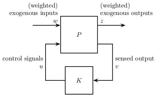
Figure 40: General Control Configuration
7 Plant Analysis
7.1 Load Plant
load('mat/plant.mat', 'G');
7.2 RGA-Number
freqs = logspace(2, 4, 1000);
G_resp = freqresp(G, freqs, 'Hz');
A = zeros(size(G_resp));
RGAnum = zeros(1, length(freqs));

for i = 1:length(freqs)
  A(:, :, i) = G_resp(:, :, i).*inv(G_resp(:, :, i))';
  RGAnum(i) = sum(sum(abs(A(:, :, i)-eye(2))));
end
% RGA = G0.*inv(G0)';
figure;
plot(freqs, RGAnum);
set(gca, 'xscale', 'log');
U = zeros(2, 2, length(freqs));
S = zeros(2, 2, length(freqs))
V = zeros(2, 2, length(freqs));

for i = 1:length(freqs)
  [Ui, Si, Vi] = svd(G_resp(:, :, i));
  U(:, :, i) = Ui;
  S(:, :, i) = Si;
  V(:, :, i) = Vi;
end
7.3 Rotation Matrix
G0 = freqresp(G, 0);
8 Active Damping
8.1 Load Plant
load('mat/plant.mat', 'sys', 'Gi', 'Zc', 'Ga', 'Gc', 'Gn', 'Gd');
8.2 Integral Force Feedback
bode(sys({'Vch', 'Vcv'}, {'Uch', 'Ucv'}));
Kppf = blkdiag(-10000/s, tf(0));

Kppf.InputName  = {'Vch', 'Vcv'};
Kppf.OutputName = {'Uch', 'Ucv'};
inputs  = {'Uch', 'Ucv', 'Unh', 'Unv'};
outputs = {'Ich', 'Icv', 'Rh', 'Rv', 'Vph', 'Vpv'};

sys_cl = connect(sys, Kppf, inputs, outputs);

figure; bode(sys_cl({'Vph', 'Vpv'}, {'Uch', 'Ucv'}), sys({'Vph', 'Vpv'}, {'Uch', 'Ucv'}))
8.3 Conclusion
Active damping does not seems to be applicable here.
9 Decentralized Control of the Sercalo
9.1 Load Plant
load('mat/plant.mat', 'sys', 'Gi', 'Zc', 'Ga', 'Gc', 'Gn', 'Gd');
9.2 Diagonal Controller
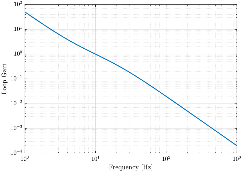
Using SISOTOOL, a diagonal controller is designed.
The two SISO loop gains are shown in Fig. 41.
Kh = -0.25598*(s+112)*(s^2 + 15.93*s + 6.686e06)/((s^2*(s+352.5)*(1+s/2/pi/2000)));
Kv = 10207*(s+55.15)*(s^2 + 17.45*s + 2.491e06)/(s^2*(s+491.2)*(s+7695));

K = blkdiag(Kh, Kv);
K.InputName  = {'Rh', 'Rv'};
K.OutputName = {'Uch', 'Ucv'};

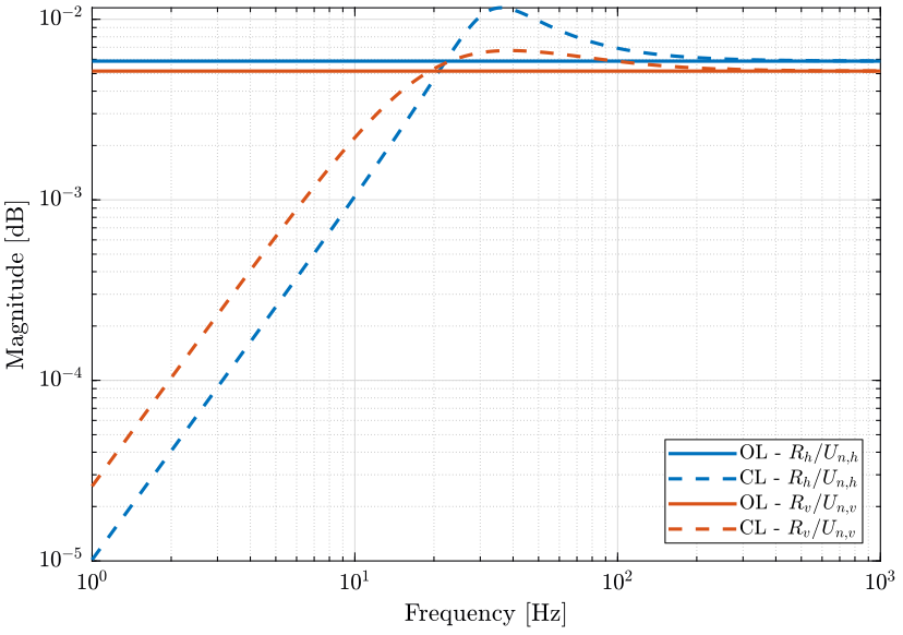
We then close the loop and we look at the transfer function from the Newport rotation signal to the beam angle (Fig. 42).
inputs  = {'Uch', 'Ucv', 'Unh', 'Unv'};
outputs = {'Vch', 'Vcv', 'Ich', 'Icv', 'Rh', 'Rv', 'Vph', 'Vpv'};

sys_cl = connect(sys, -K, inputs, outputs);
9.3 Save the Controller
Kd = c2d(K, 1e-4, 'tustin');
The diagonal controller is accessible here.
save('mat/K_diag.mat', 'K', 'Kd');
10 Newport Control
In this section, we try to implement a simple decentralized controller for the Newport. This can be used to align the 4QD:
- once there is a signal from the 4QD, the Newport feedback loop is closed
- thus, the Newport is positioned such that the beam hits the center of the 4QD
- then we can move the 4QD manually in X-Y plane in order to cancel the command signal of the Newport
- finally, we are sure to be aligned when the command signal of the Newport is 0
10.1 Load Plant
load('mat/plant.mat', 'Gn', 'Gd');
10.2 Analysis
The plant is basically a constant until frequencies up to the required bandwidth.
We get that constant value.
Gn0 = freqresp(inv(Gd)*Gn, 0);
We design two controller containing 2 integrators and one lead near the crossover frequency set to 10Hz.
h = 2;
w0 = 2*pi*10;

Knh = 1/Gn0(1,1) * (w0/s)^2 * (1 + s/w0*h)/(1 + s/w0/h)/h;
Knv = 1/Gn0(2,2) * (w0/s)^2 * (1 + s/w0*h)/(1 + s/w0/h)/h;
10.3 Save
Kn = blkdiag(Knh, Knv);
Knd = c2d(Kn, 1e-4, 'tustin');
The controllers can be downloaded here.
save('mat/K_newport.mat', 'Kn', 'Knd');
11 Measurement of the non-repeatability
The goal here is the measure the non-repeatability of the setup.
All sources of error (detailed in the budget error in Section 4) will contribute to the non-repeatability of the system.
11.1 Data Load and pre-processing
uh = load('mat/data_rep_h.mat', ...
     't', 'Uch', 'Ucv', ...
     'Unh', 'Unv', ...
     'Vph', 'Vpv', ...
     'Vnh', 'Vnv', ...
     'Va');

uv = load('mat/data_rep_v.mat', ...
     't', 'Uch', 'Ucv', ...
     'Unh', 'Unv', ...
     'Vph', 'Vpv', ...
     'Vnh', 'Vnv', ...
     'Va');
% Let's start one second after the first command in the system
i0 = find(uh.Unh ~= 0, 1) + fs;
iend = i0+fs*floor((length(uh.t)-i0)/fs);

uh.Uch([1:i0-1, iend:end]) = [];
uh.Ucv([1:i0-1, iend:end]) = [];
uh.Unh([1:i0-1, iend:end]) = [];
uh.Unv([1:i0-1, iend:end]) = [];
uh.Vph([1:i0-1, iend:end]) = [];
uh.Vpv([1:i0-1, iend:end]) = [];
uh.Vnh([1:i0-1, iend:end]) = [];
uh.Vnv([1:i0-1, iend:end]) = [];
uh.Va ([1:i0-1, iend:end]) = [];
uh.t  ([1:i0-1, iend:end]) = [];

% We reset the time t
uh.t = uh.t - uh.t(1);
% Let's start one second after the first command in the system
i0 = find(uv.Unv ~= 0, 1) + fs;
iend = i0+fs*floor((length(uv.t)-i0)/fs);

uv.Uch([1:i0-1, iend:end]) = [];
uv.Ucv([1:i0-1, iend:end]) = [];
uv.Unh([1:i0-1, iend:end]) = [];
uv.Unv([1:i0-1, iend:end]) = [];
uv.Vph([1:i0-1, iend:end]) = [];
uv.Vpv([1:i0-1, iend:end]) = [];
uv.Vnh([1:i0-1, iend:end]) = [];
uv.Vnv([1:i0-1, iend:end]) = [];
uv.Va ([1:i0-1, iend:end]) = [];
uv.t  ([1:i0-1, iend:end]) = [];

% We reset the time t
uv.t = uv.t - uv.t(1);
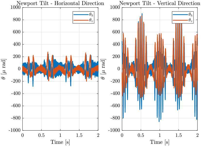
11.2 Some Time domain plots

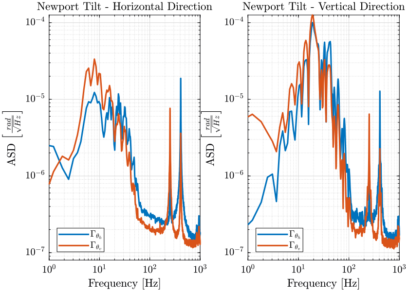
11.3 Verify Tracking Angle Error
Let’s verify that the positioning error of the beam is small and what could be the effect on the distance measured by the intereferometer.
load('./mat/plant.mat', 'Gd');
Let’s compute the PSD of the error to see the frequency content.
[psd_UhRh, f] = pwelch(uh.Vph/freqresp(Gd(1,1), 0), hanning(ceil(1*fs)), [], [], fs);
[psd_UhRv, ~] = pwelch(uh.Vpv/freqresp(Gd(2,2), 0), hanning(ceil(1*fs)), [], [], fs);
[psd_UvRh, ~] = pwelch(uv.Vph/freqresp(Gd(1,1), 0), hanning(ceil(1*fs)), [], [], fs);
[psd_UvRv, ~] = pwelch(uv.Vpv/freqresp(Gd(2,2), 0), hanning(ceil(1*fs)), [], [], fs);
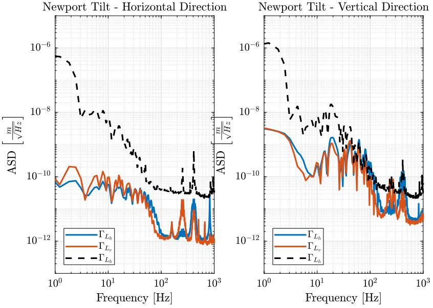
Let’s convert that to errors in distance
\[ \Delta L = L^\prime - L = \frac{L}{\cos(\alpha)} - L \approx \frac{L \alpha^2}{2} \] with
- \(L\) is the nominal distance traveled by the beam
- \(L^\prime\) is the distance traveled by the beam with an angle error
- \(\alpha\) is the angle error
L = 0.1; % [m]
[psd_UhLh, f] = pwelch(0.5*L*(uh.Vph/freqresp(Gd(1,1), 0)).^2, hanning(ceil(1*fs)), [], [], fs);
[psd_UhLv, ~] = pwelch(0.5*L*(uh.Vpv/freqresp(Gd(2,2), 0)).^2, hanning(ceil(1*fs)), [], [], fs);
[psd_UvLh, ~] = pwelch(0.5*L*(uv.Vph/freqresp(Gd(1,1), 0)).^2, hanning(ceil(1*fs)), [], [], fs);
[psd_UvLv, ~] = pwelch(0.5*L*(uv.Vpv/freqresp(Gd(2,2), 0)).^2, hanning(ceil(1*fs)), [], [], fs);
Now, compare that with the PSD of the measured distance by the interferometer (Fig. 47).
[psd_Lh, f] = pwelch(uh.Va, hanning(ceil(1*fs)), [], [], fs);
[psd_Lv, ~] = pwelch(uv.Va, hanning(ceil(1*fs)), [], [], fs);
![]()
Figure 47: Comparison of the effect of tracking error on the measured distance and the measured distance by the Attocube (png, pdf)
The tracking errors are a limiting factor.
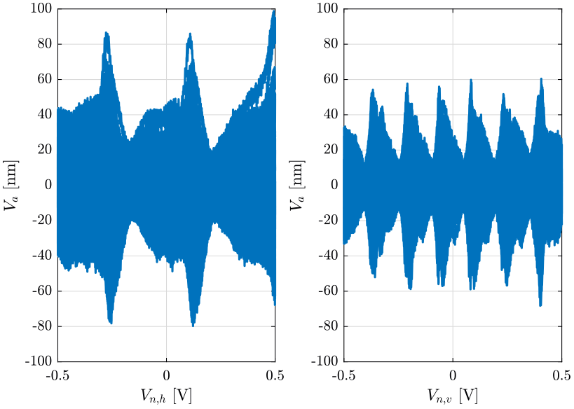
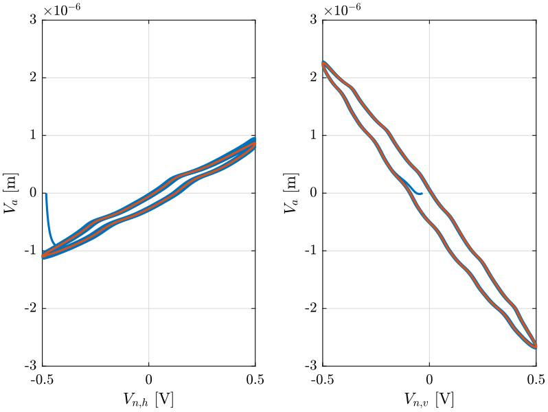
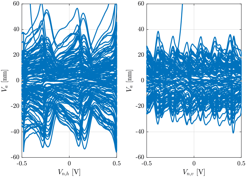
11.4 Processing
First, we get the mean value as measured by the interferometer for each value of the Newport angle.
Vahm = mean(reshape(uh.Va, [fs floor(length(uh.t)/fs)]),2);
Unhm = mean(reshape(uh.Unh, [fs floor(length(uh.t)/fs)]),2);

Vavm = mean(reshape(uv.Va, [fs floor(length(uv.t)/fs)]),2);
Unvm = mean(reshape(uv.Unv, [fs floor(length(uv.t)/fs)]),2);
And we can compute the RMS value of the non-repeatable part:
| Va - Horizontal [nm rms] | Va - Vertical [nm rms] |
|---|---|
| 19.6 | 13.9 |

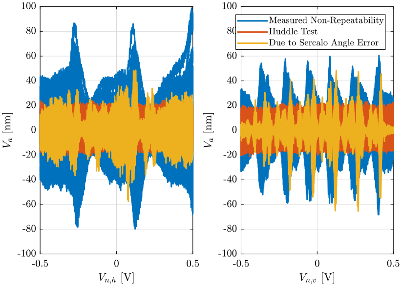
11.5 Analysis of the non-repeatable contributions
Let’s know try to determine where does the non-repeatability comes from.
From the 4QD signal, we can compute the angle error of the beam and thus determine the corresponding displacement measured by the attocube.
We then take the non-repeatable part of this displacement and we compare that with the total non-repeatability.
We also plot the displacement measured during the huddle test.
All the signals are shown on Fig. 50.
11.6 Results with a low pass filter
We filter the data with a first order low pass filter with a crossover frequency of \(\omega_0\).
w0 = 10; % [Hz]

G_lpf = 1/(1 + s/2/pi/w0);

uh.Vaf = lsim(G_lpf, uh.Va, uh.t);
uv.Vaf = lsim(G_lpf, uv.Va, uv.t);
11.7 Processing
First, we get the mean value as measured by the interferometer for each value of the Newport angle.
Vahm = mean(reshape(uh.Vaf, [fs floor(length(uh.t)/fs)]),2);
Unhm = mean(reshape(uh.Unh, [fs floor(length(uh.t)/fs)]),2);

Vavm = mean(reshape(uv.Vaf, [fs floor(length(uv.t)/fs)]),2);
Unvm = mean(reshape(uv.Unv, [fs floor(length(uv.t)/fs)]),2);
And we can compute the RMS value of the non-repeatable part:
| Va - Horizontal [nm rms] | Va - Vertical [nm rms] |
|---|---|
| 22.9 | 13.9 |