A brief and practical introduction to \(\mathcal{H}_\infty\) Control
Table of Contents
- Introduction
- 1. Introduction to Model Based Control
- 2. Classical Open Loop Shaping
- 3. A first Step into the \(\mathcal{H}_\infty\) world
- 4. Modern Interpretation of Control Specifications
- 5. \(\mathcal{H}_\infty\) Shaping of closed-loop transfer functions
- 6. Mixed-Sensitivity \(\mathcal{H}_\infty\) Control - Example
- 7. Conclusion
This document is also available as a pdf.
Introduction
The purpose of this document is to give a practical introduction to the wonderful world of \(\mathcal{H}_\infty\) Control.
No attend is made to provide an exhaustive treatment of the subject. \(\mathcal{H}_\infty\) Control is a very broad topic and entire books are written on it. Therefore, for more advanced discussion, please have a look at the recommended references at the bottom of this document.
When possible, Matlab scripts used for the example/exercises are provided such that you can easily test them on your computer.
The general structure of this document is as follows:
- A short introduction to model based control is given in Section 1
- Classical open loop shaping method is presented in Section 2. It is also shown that \(\mathcal{H}_\infty\) synthesis can be used for open loop shaping
- Important concepts indispensable for \(\mathcal{H}_\infty\) control such as the \(\mathcal{H}_\infty\) norm and the generalized plant are introduced in Section 3
- A very important step in \(\mathcal{H}_\infty\) control is to express the control specifications (performances, robustness, etc.) as an \(\mathcal{H}_\infty\) optimization problem. Such procedure is described in Section 4
- One of the most useful use of the \(\mathcal{H}_\infty\) control is the shaping of closed-loop transfer functions. Such technique is presented in Section 5
- Finally, complete examples of the use of \(\mathcal{H}_\infty\) Control for practical problems are provided in Section 6
1 Introduction to Model Based Control
1.1 Model Based Control - Methodology
The typical methodology for Model Based Control techniques is schematically shown in Figure 1.
It consists of three steps:
- Identification or modeling: a mathematical model \(G(s)\) representing the plant dynamics is obtained
- Translate the specifications into mathematical criteria:
- Specifications: Response Time, Noise Rejection, Maximum input amplitude, Robustness, …
- Mathematical Criteria: Cost Function, Shape of transfer function, Phase/Gain margin, Roll-Off, …
- Synthesis: research of a controller \(K(s)\) that satisfies the specifications for the model of the system
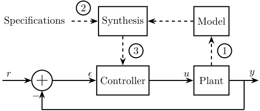
Figure 1: Typical Methodoly for Model Based Control
In this document, we will suppose a model of the plant is available (step 1 already performed), and we will focus on steps 2 and 3.
In Section 2, steps 2 and 3 will be described for a control techniques called classical (open-)loop shaping.
Then, steps 2 and 3 for the \(\mathcal{H}_\infty\) Loop Shaping of closed-loop transfer functions will be discussed in Sections 4, 5 and 6.
1.2 From Classical Control to Robust Control
Many different model based control techniques have been developed since the birth of classical control theory in the ’30s.
Classical control methods were developed starting from 1930 based on tools such as the Laplace and Fourier transforms. It was then natural to study systems in the frequency domain using tools such as the Bode and Nyquist plots. Controllers were manually tuned to optimize criteria such as control bandwidth, gain and phase margins.
The ’60s saw the development of control techniques based on a state-space. Linear algebra and matrices were used instead of the frequency domain tool of the class control theory. This allows multi-inputs multi-outputs systems to be easily treated. Kalman introduced the well known Kalman estimator as well the notion of optimality by minimizing quadratic cost functions. This set of developments is loosely termed Modern Control theory.
By the 1980’s, modern control theory was shown to have some robustness issues and to lack the intuitive tools that the classical control methods were offering. This led to a new control theory called Robust control that blends the best features of classical and modern techniques. This robust control theory is the subject of this document.
The three presented control methods are compared in Table 1.
Note that in parallel, there have been numerous other developments, including non-linear control, adaptive control, machine-learning control just to name a few.
| Classical Control | Modern Control | Robust Control | |
|---|---|---|---|
| Date | 1930- | 1960- | 1980- |
| Tools | Transfer Functions | State Space formulation | Systems/Signal Norms |
| Nyquist, Bode Plots | Riccati Equations | Closed Loop TF | |
| Root Locus | Kalman Filters | Closed Loop Shaping | |
| Phase/Gain margins | Weighting Functions | ||
| Open Loop Shaping | Disk margin | ||
| Controllers | P, PI, PID | Full State Feedback | General Control Conf. |
| Leads, Lags | LQG, LQR | ||
| Advantages | Study Stability | Automatic Synthesis | Automatic Synthesis |
| Simple | MIMO | MIMO | |
| Natural | Optimization Problem | Optimization Problem | |
| Guaranteed Robustness | |||
| Disadvant. | Manual Method | No Guaranteed Robustness | Requires knowledge of tools |
| Only SISO | Rejection of Pert. | Need good model of the system | |
| No input usage lim. |
1.3 Example System
Throughout this document, multiple examples and practical application of presented control strategies will be provided. Most of them will be applied on a physical system presented in this section.
This system is shown in Figure 2. It could represent an active suspension stage supporting a payload. The inertial motion of the payload is measured using an inertial sensor and this is feedback to a force actuator. Such system could be used to actively isolate the payload (disturbance rejection problem) or to make it follow a trajectory (tracking problem).
The notations used on Figure 2 are listed and described in Table 2.
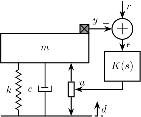
Figure 2: Test System consisting of a payload with a mass \(m\) on top of an active system with a stiffness \(k\), damping \(c\) and an actuator. A feedback controller \(K(s)\) is added to position / isolate the payload.
| Notation | Description | Value | Unit |
|---|---|---|---|
| \(m\) | Payload’s mass to position / isolate | \(10\) | [kg] |
| \(k\) | Stiffness of the suspension system | \(10^6\) | [N/m] |
| \(c\) | Damping coefficient of the suspension system | \(400\) | [N/(m/s)] |
| \(y\) | Payload absolute displacement (measured by an inertial sensor) | [m] | |
| \(d\) | Ground displacement, it acts as a disturbance | [m] | |
| \(u\) | Actuator force | [N] | |
| \(r\) | Wanted position of the mass (the reference) | [m] | |
| \(\epsilon = r - y\) | Position error | [m] | |
| \(K\) | Feedback controller | to be designed | [N/m] |
Derive the following open-loop transfer functions:
\begin{align} G(s) &= \frac{y}{u} \\ G_d(s) &= \frac{y}{d} \end{align}Hint
You can follow this generic procedure:
- List all applied forces ot the mass: Actuator force, Stiffness force (Hooke’s law), …
- Apply the Newton’s Second Law on the payload \[ m \ddot{y} = \Sigma F \]
- Transform the differential equations into the Laplace domain: \[ \frac{d\ \cdot}{dt} \Leftrightarrow \cdot \times s \]
- Write \(y(s)\) as a function of \(u(s)\) and \(w(s)\)
Results
\begin{align} G(s) &= \frac{1}{m s^2 + cs + k} \\ G_d(s) &= \frac{cs + k}{m s^2 + cs + k} \end{align}Having obtained \(G(s)\) and \(G_d(s)\), we can transform the system shown in Figure 2 into a classical feedback architecture as shown in Figure 6.
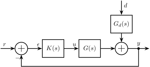
Figure 3: Block diagram corresponding to the example system of Figure 2
Let’s define the system parameters on Matlab.
1: k = 1e6; % Stiffness [N/m]
2: c = 4e2; % Damping [N/(m/s)]
3: m = 10; % Mass [kg]
And now the system dynamics \(G(s)\) and \(G_d(s)\).
4: G = 1/(m*s^2 + c*s + k); % Plant
5: Gd = (c*s + k)/(m*s^2 + c*s + k); % Disturbance
The Bode plots of \(G(s)\) and \(G_d(s)\) are shown in Figures 4 and 5.
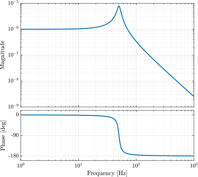
Figure 4: Bode plot of the plant \(G(s)\)
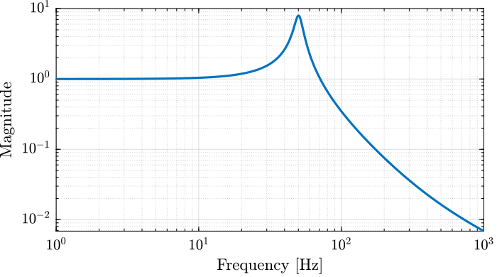
Figure 5: Magnitude of the disturbance transfer function \(G_d(s)\)
2 Classical Open Loop Shaping
After an introduction to classical Loop Shaping in Section 2.1, a practical example is given in Section 2.2. Such Loop Shaping is usually performed manually with tools coming from the classical control theory.
However, the \(\mathcal{H}_\infty\) synthesis can be used to automate the Loop Shaping process. This is presented in Section 2.3 and applied on the same example in Section 2.4.
2.1 Introduction to Loop Shaping
Loop Shaping refers to a control design procedure that involves explicitly shaping the magnitude of the Loop Transfer Function \(L(s)\).
The Loop Gain (or Loop transfer function) \(L(s)\) usually refers to as the product of the controller and the plant (see Figure 6):
\begin{equation} L(s) = G(s) \cdot K(s) \label{eq:loop_gain} \end{equation}Its name comes from the fact that this is actually the “gain around the loop”.
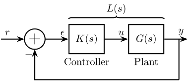
Figure 6: Classical Feedback Architecture
This synthesis method is one of main way controllers are design in the classical control theory. It is widely used and generally successful as many characteristics of the closed-loop system depend on the shape of the open loop gain \(L(s)\) such as:
- Good Tracking: \(L\) large
- Good disturbance rejection: \(L\) large
- Attenuation of measurement noise on plant output: \(L\) small
- Small magnitude of input signal: \(L\) small
- Nominal stability: \(L\) small (RHP zeros and time delays)
- Robust stability: \(L\) small (neglected dynamics)
The shaping of the Loop Gain is done manually by combining several leads, lags, notches… This process is very much simplified by the fact that the loop gain \(L(s)\) depends linearly on \(K(s)\) \eqref{eq:loop_gain}. A typical wanted Loop Shape is shown in Figure 7. Another interesting Loop shape called “Bode Step” is described in [1].
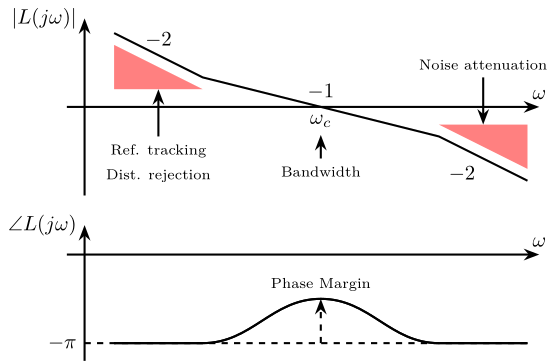
Figure 7: Typical Wanted Shape for the Loop Gain \(L(s)\)
The shaping of closed-loop transfer functions is obviously not as simple as they don’t depend linearly on \(K(s)\). But this is were the \(\mathcal{H}_\infty\) Synthesis will be useful! More details on that in Sections 4 and 5.
2.2 Example of Manual Open Loop Shaping
Let’s take our example system described in Section 1.3 and design a controller using the Open-Loop shaping synthesis approach. The specifications are:
- Disturbance rejection: Highest possible rejection below 1Hz
- Positioning speed: Bandwidth of approximately 10Hz
- Noise attenuation: Roll-off of -40dB/decade past 30Hz
- Robustness: Gain margin > 3dB and Phase margin > 30 deg
Using SISOTOOL, design a controller that fulfills the specifications.
sisotool(G)
Hint
You can follow this procedure:
- In order to have good disturbance rejection at low frequency, add a simple or double integrator
- In terms of the loop gain, the bandwidth can be defined at the frequency \(\omega_c\) where \(|l(j\omega_c)|\) first crosses 1 from above. Therefore, adjust the gain such that \(L(j\omega)\) crosses 1 at around 10Hz
- The roll-off at high frequency for noise attenuation should already be good enough. If not, add a low pass filter
- Add a Lead centered around the crossover frequency (10 Hz) and tune it such that sufficient phase margin is added. Verify that the gain margin is good enough.
Let’s say we came up with the following controller.
K = 14e8 * ...              % Gain
    1/(s^2) * ...           % Double Integrator
    1/(1 + s/2/pi/40) * ... % Low Pass Filter
    (1 + s/(2*pi*10/sqrt(8)))/(1 + s/(2*pi*10*sqrt(8))); % Lead
The bode plot of the Loop Gain is shown in Figure 8 and we can verify that we have the wanted stability margins using the margin command:
[Gm, Pm, ~, Wc] = margin(G*K)
| Requirements | Manual Method |
|---|---|
| Gain Margin \(> 3\) [dB] | 3.1 |
| Phase Margin \(> 30\) [deg] | 35.4 |
| Crossover \(\approx 10\) [Hz] | 10.1 |
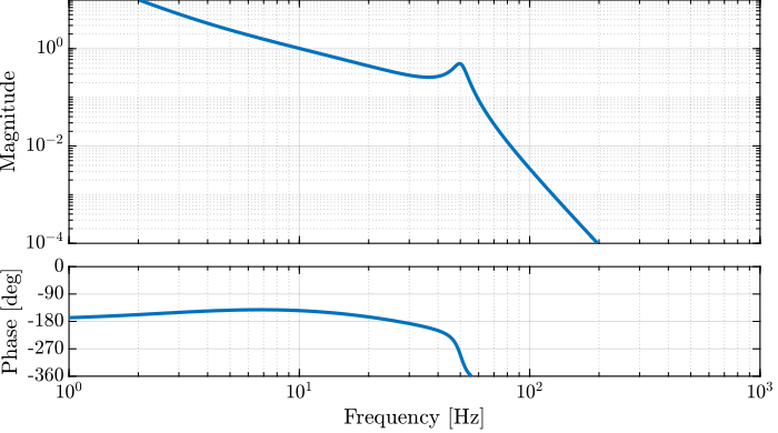
Figure 8: Bode Plot of the obtained Loop Gain \(L(s) = G(s) K(s)\)
2.3 \(\mathcal{H}_\infty\) Loop Shaping Synthesis
The synthesis of controllers based on the Loop Shaping method can be automated using the \(\mathcal{H}_\infty\) Synthesis.
Using Matlab, it can be easily performed using the loopsyn command:
K = loopsyn(G, Lw);
where:
Gis the (LTI) plantLwis the wanted loop shapeKis the synthesize controller
Matlab documentation of loopsyn (link).
Therefore, by just providing the wanted loop shape and the plant model, the \(\mathcal{H}_\infty\) Loop Shaping synthesis generates a stabilizing controller such that the obtained loop gain \(L(s)\) matches the specified one with an accuracy \(\gamma\).
Even though we will not go into details and explain how such synthesis is working, an example is provided in the next section.
2.4 Example of the \(\mathcal{H}_\infty\) Loop Shaping Synthesis
To apply the \(\mathcal{H}_\infty\) Loop Shaping Synthesis, the wanted shape of the loop gain should be determined from the specifications. This is summarized in Table 3.
Such shape corresponds to the typical wanted Loop gain Shape shown in Figure 7.
| Specification | Corresponding Loop Shape | |
|---|---|---|
| Dist. Rej. | Highest possible rejection below 1Hz | Slope of -40dB/dec at low frequency |
| Pos. Speed | Bandwidth of approximately 10Hz | \(L\) crosses 1 at 10Hz |
| Noise Att. | Roll-off of -40dB/decade past 30Hz | Roll-off of -40dB/decade past 30Hz |
| Robustness | \(\Delta G > 3dB\), \(\Delta \phi > 30^o\) | Slope of -20dB/decade near the crossover |
Then, a (stable, minimum phase) transfer function \(L_w(s)\) should be created that has the same gain as the wanted shape of the Loop gain. For this example, a double integrator and a lead centered on 10Hz are used. Then the gain is adjusted such that the \(|L_w(j2 \pi 10)| = 1\).
Using Matlab, we have:
Lw = 2.3e3 * ...
     1/(s^2) * ... % Double Integrator
     (1 + s/(2*pi*10/sqrt(3)))/(1 + s/(2*pi*10*sqrt(3))); % Lead
The \(\mathcal{H}_\infty\) open loop shaping synthesis is then performed using the loopsyn command:
[K, ~, GAM] = loopsyn(G, Lw);
The obtained Loop Gain is shown in Figure 9 and matches the specified one by a factor \(\gamma \approx 2\).
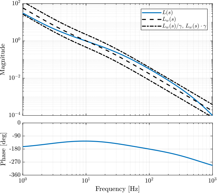
Figure 9: Obtained Open Loop Gain \(L(s) = G(s) K(s)\) and comparison with the wanted Loop gain \(L_w\)
When using the \(\mathcal{H}_\infty\) Synthesis, it is usually recommended to analyze the obtained controller.
This is usually done by breaking down the controller into simple elements such as low pass filters, high pass filters, notches, leads, etc.
Let’s briefly analyze the obtained controller which bode plot is shown in Figure 10:
- two integrators are used at low frequency to have the wanted low frequency high gain
- a lead is added centered with the crossover frequency to increase the phase margin
- a notch is added at the resonance of the plant to increase the gain margin (this is very typical of \(\mathcal{H}_\infty\) controllers, and can be an issue, more info on that latter)
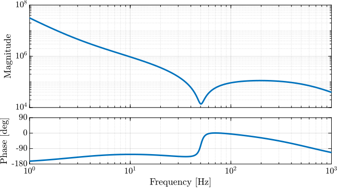
Figure 10: Obtained controller \(K\) using the open-loop \(\mathcal{H}_\infty\) shaping
Let’s finally compare the obtained stability margins of the \(\mathcal{H}_\infty\) controller and of the manually developed controller in Table 4.
| Specifications | Manual Method | \(\mathcal{H}_\infty\) Method |
|---|---|---|
| Gain Margin \(> 3\) [dB] | 3.1 | 31.7 |
| Phase Margin \(> 30\) [deg] | 35.4 | 54.7 |
| Crossover \(\approx 10\) [Hz] | 10.1 | 9.9 |
3 A first Step into the \(\mathcal{H}_\infty\) world
In this section, the \(\mathcal{H}_\infty\) Synthesis method, which is based on the optimization of the \(\mathcal{H}_\infty\) norm of transfer functions, is introduced.
After the \(\mathcal{H}_\infty\) norm is defined in Section 3.1, the \(\mathcal{H}_\infty\) synthesis procedure is described in Section 3.2 .
The generalized plant, a very useful tool to describe a control problem, is presented in Section 3.3. The \(\mathcal{H}_\infty\) is then applied to this generalized plant in Section 3.4.
Finally, an example showing how to convert a typical feedback control architecture into a generalized plant is given in Section 3.5.
3.1 The \(\mathcal{H}_\infty\) Norm
The \(\mathcal{H}_\infty\) norm of a multi-input multi-output system \(G(s)\) is defined as the peak of the maximum singular value of its frequency response
\begin{equation} \|G(s)\|_\infty = \max_\omega \bar{\sigma}\big( G(j\omega) \big) \end{equation}For a single-input single-output system \(G(s)\), it is simply the peak value of \(|G(j\omega)|\) as a function of frequency:
\begin{equation} \|G(s)\|_\infty = \max_{\omega} |G(j\omega)| \label{eq:hinf_norm_siso} \end{equation}
Let’s compute the \(\mathcal{H}_\infty\) norm of our test plant \(G(s)\) using the hinfnorm function:
hinfnorm(G)
7.9216e-06
We can see in Figure 11 that indeed, the \(\mathcal{H}_\infty\) norm of \(G(s)\) does corresponds to the peak value of \(|G(j\omega)|\).
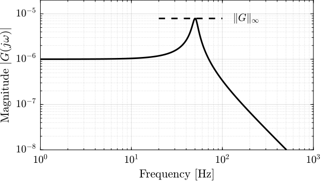
Figure 11: Example of the \(\mathcal{H}_\infty\) norm of a SISO system
3.2 \(\mathcal{H}_\infty\) Synthesis
The \(\mathcal{H}_\infty\) synthesis is a method that uses an algorithm (LMI optimization, Riccati equation) to find a controller that stabilizes the system and that minimizes the \(\mathcal{H}_\infty\) norms of defined transfer functions.
Why optimizing the \(\mathcal{H}_\infty\) norm of transfer functions is a pertinent choice will become clear when we will translate the typical control specifications into the \(\mathcal{H}_\infty\) norm of transfer functions in Section 4.
Then applying the \(\mathcal{H}_\infty\) synthesis to a plant, the engineer work usually consists of the following steps:
- Write the problem as standard \(\mathcal{H}_\infty\) problem using the generalized plant (described in the next section)
- Translate the specifications as \(\mathcal{H}_\infty\) norms of transfer functions (Section 4)
- Make the synthesis and analyze the obtained controller
As the \(\mathcal{H}_\infty\) synthesis usually gives very high order controllers, an additional step that reduces the controller order is sometimes required for practical implementation.
Note that there are many ways to use the \(\mathcal{H}_\infty\) Synthesis:
3.3 The Generalized Plant
The first step when applying the \(\mathcal{H}_\infty\) synthesis is usually to write the problem as a standard \(\mathcal{H}_\infty\) problem. This consist of deriving the Generalized Plant for the current problem.
The generalized plant, usually noted \(P(s)\), is shown in Figure 12. It has two sets of inputs \([w,\,u]\) and two sets of outputs \([z\,v]\) such that:
\begin{equation} \begin{bmatrix} z \\ v \end{bmatrix} = P \begin{bmatrix} w \\ u \end{bmatrix} \end{equation}The meaning of these inputs and outputs are summarized in Table 5.
A practical example about how to derive the generalized plant for a classical control problem is given in Section 3.5.
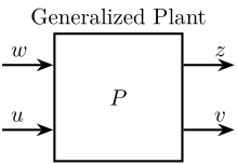
Figure 12: Inputs and Outputs of the generalized Plant
| Notation | Meaning |
|---|---|
| \(P\) | Generalized plant model |
| \(w\) | Exogenous inputs: references, disturbances, noises |
| \(z\) | Exogenous outputs: signals to be minimized |
| \(v\) | Controller inputs: measurements |
| \(u\) | Control signals |
3.4 The \(\mathcal{H}_\infty\) Synthesis applied on the Generalized plant
Once the generalized plant is obtained, the \(\mathcal{H}_\infty\) synthesis problem can be stated as follows:
- \(\mathcal{H}_\infty\) Synthesis applied on the generalized plant
Find a stabilizing controller \(K\) that, using the sensed outputs \(v\), generates control signals \(u\) such that the \(\mathcal{H}_\infty\) norm of the closed-loop transfer function from \(w\) to \(z\) is minimized.
After \(K\) is found, the system is robustified by adjusting the response around the unity gain frequency to increase stability margins.
The obtained controller \(K\) and the generalized plant are connected as shown in Figure 13.
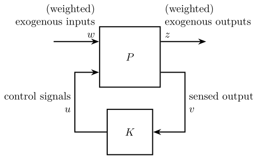
Figure 13: General Control Configuration
Using Matlab, the \(\mathcal{H}_\infty\) Synthesis applied on a Generalized plant can be applied using the hinfsyn command (documentation):
K = hinfsyn(P, nmeas, ncont);
where:
Pis the generalized plant transfer function matrixnmeasis the number of sensed output (size of \(v\))ncontis the number of control signals (size of \(u\))Kobtained controller (of sizencont x nmeas) that minimizes the \(\mathcal{H}_\infty\) norm from \(w\) to \(z\).
Note that the general control configure of Figure 13, as its name implies, is quite general and can represent feedback control as well as feedforward control architectures.
3.5 From a Classical Feedback Architecture to a Generalized Plant
The procedure to convert a typical control architecture as the one shown in Figure 14 to a generalized Plant is as follows:
- Define signals of the generalized plant: \(w\), \(z\), \(u\) and \(v\)
- Remove \(K\) and rearrange the inputs and outputs to match the generalized configuration shown in Figure 12
Consider the feedback control architecture shown in Figure 14. Suppose we want to design \(K\) using the general \(\mathcal{H}_\infty\) synthesis, and suppose the signals to be minimized are the control input \(u\) and the tracking error \(\epsilon\).
- Convert the control architecture to a generalized configuration
- Compute the transfer function matrix of the generalized plant \(P\) using Matlab as a function or \(K\) and \(G\)
![]()
Figure 14: Classical Feedback Control Architecture (Tracking)
Hint
First, define the signals of the generalized plant:
- Exogenous inputs: \(w = r\)
- Signals to be minimized: Usually, we want to minimize the tracking errors \(\epsilon\) and the control signal \(u\): \(z = [\epsilon,\ u]\)
- Controller inputs: this is the signal at the input of the controller: \(v = \epsilon\)
- Controller outputs: signal generated by the controller: \(u\)
Then, Remove \(K\) and rearrange the inputs and outputs as in Figure 12.
Answer
The obtained generalized plant shown in Figure 15.
![]()
Figure 15: Generalized plant of the Classical Feedback Control Architecture (Tracking)
Using Matlab, the generalized plant can be defined as follows:
P = [1 -G;
     0  1;
     1 -G]
P.InputName = {'w', 'u'};
P.OutputName = {'e', 'u', 'v'};
4 Modern Interpretation of Control Specifications
As shown in Section 2, the loop gain \(L(s) = G(s) K(s)\) is a useful and easy tool when manually designing controllers. This is mainly due to the fact that \(L(s)\) is very easy to shape as it depends linearly on \(K(s)\). Moreover, important quantities such as the stability margins and the control bandwidth can be estimated from the shape/phase of \(L(s)\).
However, the loop gain \(L(s)\) does not directly give the performances of the closed-loop system. As a matter of fact, the behavior of the closed-loop system by the closed-loop transfer functions. These are derived of a typical feedback architecture functions in Section 4.1.
The modern interpretation of control specifications then consists of determining the required shape of the closed-loop transfer functions such that the system behavior corresponds to the requirements. Once this is done, the \(\mathcal{H}_\infty\) synthesis can be used to generate a controller that will shape the closed-loop transfer function as specified.. This method is presented in Section 5.
One of the most important closed-loop transfer function is called the sensitivity function. Its link with the closed-loop behavior of the feedback system is studied in Section 4.2.
The robustness (stability margins) of the system can also be linked to the shape of the sensitivity function with the use of the module margin (Section 4.3).
Links between typical control specifications and shapes of the closed-loop transfer functions are summarized in Section 4.4.
4.1 Closed Loop Transfer Functions and the Gang of Four
Consider the typical feedback system shown in Figure 16.
The behavior (performances) of this feedback system is determined by the closed-loop transfer functions from the inputs (\(r\), \(d\) and \(n\)) to the important signals such as \(\epsilon\), \(u\) and \(y\).
Depending on the specification, different closed-loop transfer functions do matter. These are summarized in Table 6.
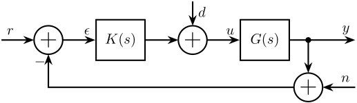
Figure 16: Simple Feedback Architecture with \(r\) the reference signal, \(\epsilon\) the tracking error, \(d\) a disturbance acting at the plant input \(u\), \(y\) is the output signal and \(n\) the measurement noise
| Specification | CL Transfer Function |
|---|---|
| Reference Tracking | From \(r\) to \(\epsilon\) |
| Disturbance Rejection | From \(d\) to \(y\) |
| Measurement Noise Filtering | From \(n\) to \(y\) |
| Small Command Amplitude | From \(n,r,d\) to \(u\) |
| Stability | All |
| Robustness (stability margins) | Module margin (see Section 4.3) |
For the feedback system in Figure 16, write the output signals \([\epsilon, u, y]\) as a function of the systems \(K(s), G(s)\) and the input signals \([r, d, n]\).
Hint
Take one of the output (e.g. \(y\)), and write it as a function of the inputs \([d, r, n]\) going step by step around the loop:
\begin{align*} y &= G u \\ &= G (d + K \epsilon) \\ &= G \big(d + K (r - n - y) \big) \\ &= G d + GK r - GK n - GK y \end{align*}Isolate \(y\) at the right hand side, and finally obtain: \[ y = \frac{GK}{1+ GK} r + \frac{G}{1 + GK} d - \frac{GK}{1 + GK} n \]
Do the same procedure for \(u\) and \(\epsilon\)
Answer
The following equations should be obtained:
\begin{align} y &= \frac{GK}{1 + GK} r + \frac{G}{1 + GK} d - \frac{GK}{1 + GK} n \\ \epsilon &= \frac{1 }{1 + GK} r - \frac{G}{1 + GK} d - \frac{G }{1 + GK} n \\ u &= \frac{K }{1 + GK} r - \frac{1}{1 + GK} d - \frac{K }{1 + GK} n \end{align}We can see that they are 4 different closed-loop transfer functions describing the behavior of the feedback system in Figure 16. These called the Gang of Four:
\begin{align} S &= \frac{1 }{1 + GK}, \quad \text{the sensitivity function} \\ T &= \frac{GK}{1 + GK}, \quad \text{the complementary sensitivity function} \\ GS &= \frac{G }{1 + GK}, \quad \text{the load disturbance sensitivity function} \\ KS &= \frac{K }{1 + GK}, \quad \text{the noise sensitivity function} \end{align}If a feedforward controller is included, a Gang of Six transfer functions can be defined. More on that in this short video.
The behavior of the feedback system in Figure 16 is fully described by the following set of equations:
\begin{align} \epsilon &= S r - GS d - GS n \\ y &= T r + GS d - T n \\ u &= KS r - S d - KS n \end{align}Thus, for reference tracking, we have to shape the closed-loop transfer function from \(r\) to \(\epsilon\), that is the sensitivity function \(S(s)\). Similarly, to reduce the effect of measurement noise \(n\) on the output \(y\), we have to act on the complementary sensitivity function \(T(s)\).
4.2 The Sensitivity Function
The sensitivity function is indisputably the most important closed-loop transfer function of a feedback system. In this section, we will see how the shape of the sensitivity function will impact the performances of the closed-loop system.
Suppose we have developed a “reference” controller \(K_r(s)\) and made three small changes to obtained three controllers \(K_1(s)\), \(K_2(s)\) and \(K_3(s)\). The obtained sensitivity functions for these four controllers are shown in Figure 17 and the corresponding step responses are shown in Figure 18.
The comparison of the sensitivity functions shapes and their effect on the step response is summarized in Table 7.
| Controller | Sensitivity Function Shape | Change of the Step Response |
|---|---|---|
| \(K_1(s)\) | Larger bandwidth \(\omega_b\) | Faster rise time |
| \(K_2(s)\) | Larger peak value \(\Vert S\Vert_\infty\) | Large overshoot and oscillations |
| \(K_3(s)\) | Larger low frequency gain \(\vert S(j\cdot 0)\vert\) | Larger static error |
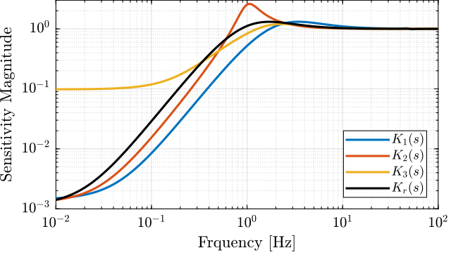
Figure 17: Sensitivity function magnitude \(|S(j\omega)|\) corresponding to the reference controller \(K_r(s)\) and the three modified controllers \(K_i(s)\)
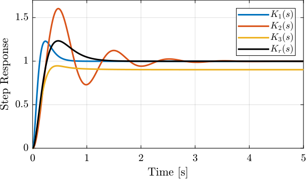
Figure 18: Step response (response from \(r\) to \(y\)) for the different controllers
- Closed-Loop Bandwidth
The closed-loop bandwidth \(\omega_b\) is the frequency where \(|S(j\omega)|\) first crosses \(1/\sqrt{2} = -3dB\) from below.
In general, a large bandwidth corresponds to a faster rise time.
From the simple analysis above, we can draw a first estimation of the wanted shape for the sensitivity function (Figure 19):
- A small magnitude at low frequency to make the static errors small
- A wanted minimum closed-loop bandwidth in order to have fast rise time and good rejection of perturbations
- A small peak value (small \(\mathcal{H}_\infty\) norm) in order to limit large overshoot and oscillations. This generally means higher robustness. This will become clear in the next section about the module margin.
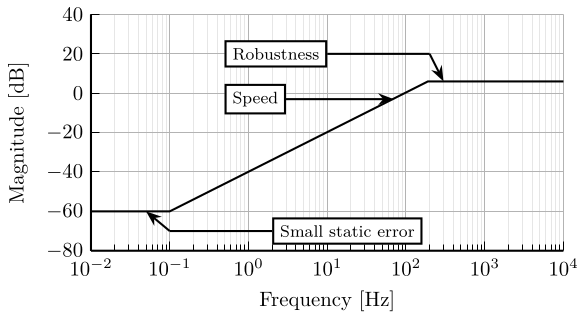
Figure 19: Typical wanted shape of the Sensitivity transfer function
4.3 Robustness: Module Margin
Let’s start this section by an example demonstrating why the phase and gain margins might not be good indicators of robustness. Will follow a discussion about the module margin, a robustness indicator that can be linked to the \(\mathcal{H}_\infty\) norm of \(S\) and that will prove to be very useful.
Consider the following plant \(G_t(s)\):
w0 = 2*pi*100;
xi = 0.1;
k = 1e7;

Gt = 1/k*(s/w0/4 + 1)/(s^2/w0^2 + 2*xi*s/w0 + 1);
Let’s say we have designed a controller \(K_t(s)\) that gives the loop gain shown in Figure 20.
Kt = 1.2e6*(s + w0)/s;
The following characteristics can be determined from the Loop gain in Figure 20:
- Control bandwidth of \(\approx 10\, \text{Hz}\)
- Infinite gain margin (the phase of the loop-gain never reaches \(-180^o\))
- More than \(90^o\) of phase margin
This clearly indicate very good robustness of the closed-loop system! Or does it? Let’s find out.
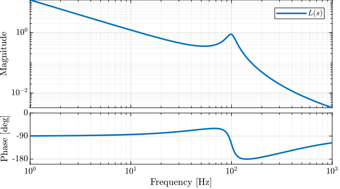
Figure 20: Bode plot of the obtained Loop Gain \(L(s)\)
Now let’s suppose the controller is implemented in practice, and the “real” plant \(G_r(s)\) as a slightly lower damping factor than the one estimated for the model:
xi = 0.03;
The obtained “real” loop gain is shown in Figure 21. At a frequency little bit above 100Hz, the phase of the loop gain reaches -180 degrees while its magnitude is more than one which indicates instability.
It is confirmed by checking the stability of the closed loop system:
isstable(feedback(Gr,K))
0
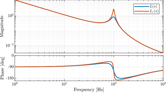
Figure 21: Bode plots of \(L(s)\) (loop gain corresponding the nominal plant) and \(L_r(s)\) (loop gain corresponding to the real plant)
Therefore, even a small change of the plant parameter renders the system unstable even though both the gain margin and the phase margin for the nominal plant are excellent.
This is due to the fact that the gain and phase margin are robustness indicators corresponding a pure change or gain or a pure change of phase but not a combination of both.
Let’s now determine a new robustness indicator based on the Nyquist Stability Criteria.
- Nyquist Stability Criteria (for stable systems)
- If the open-loop transfer function \(L(s)\) is stable, then the closed-loop system will be unstable for any encirclement of the point \(-1\) on the Nyquist plot.
- Nyquist Plot
- The Nyquist plot shows the evolution of \(L(j\omega)\) in the complex plane from \(\omega = 0 \to \infty\).
For more information about the general Nyquist Stability Criteria, you may want to look at this video.
From the Nyquist stability criteria, it is clear that we want \(L(j\omega)\) to be as far as possible from the \(-1\) point (called the unstable point) in the complex plane. This minimum distance is called the module margin.
- Module Margin
- The Module Margin \(\Delta M\) is defined as the minimum distance between the point \(-1\) and the loop gain \(L(j\omega)\) in the complex plane.
A typical Nyquist plot is shown in Figure 22. The gain, phase and module margins are graphically shown to have an idea of what they represent.
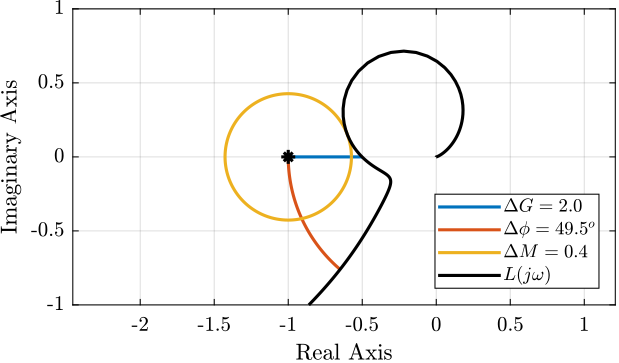
Figure 22: Nyquist plot with visual indication of the Gain margin \(\Delta G\), Phase margin \(\Delta \phi\) and Module margin \(\Delta M\)
As expected from Figure 22, there is a close relationship between the module margin and the gain and phase margins. We can indeed show that for a given value of the module margin \(\Delta M\), we have:
\begin{equation} \Delta G \ge \frac{1}{1 - \Delta M}; \quad \Delta \phi \ge \Delta M \end{equation}Let’s now try to express the Module margin \(\Delta M\) as an \(\mathcal{H}_\infty\) norm of a closed-loop transfer function:
\begin{align*} \Delta M &= \text{minimum distance between } L(j\omega) \text{ and point } (-1) \\ &= \min_\omega |L(j\omega) - (-1)| \\ &= \min_\omega |1 + L(j\omega)| \\ &= \frac{1}{\max_\omega \frac{1}{|1 + L(j\omega)|}} \\ &= \frac{1}{\max_\omega \left| \frac{1}{1 + G(j\omega)K(j\omega)}\right|} \\ &= \frac{1}{\|S\|_\infty} \end{align*}Therefore, for a given \(\mathcal{H}_\infty\) norm of \(S\) (\(\|S\|_\infty = M_S\)), we have:
\begin{equation} \Delta G \ge \frac{M_S}{M_S - 1}; \quad \Delta \phi \ge \frac{1}{M_S} \end{equation}The \(\mathcal{H}_\infty\) norm of the sensitivity function \(\|S\|_\infty\) is a measure of the Module margin \(\Delta M\) and therefore an indicator of the system robustness.
\begin{equation} \Delta M = \frac{1}{\|S\|_\infty} \label{eq:module_margin_S} \end{equation}The wanted robustness of the closed-loop system can be specified by setting a maximum value on \(\|S\|_\infty\).
Note that this is why large peak value of \(|S(j\omega)|\) usually indicate robustness problems. And we now understand why setting an upper bound on the magnitude of \(S\) is generally a good idea.
Typical, we require \(\|S\|_\infty < 2 (6dB)\) which implies \(\Delta G \ge 2\) and \(\Delta \phi \ge 29^o\)
To learn more about module/disk margin, you can check out this video.
4.4 Summary of typical specification and associated wanted shaping
| Open-Loop Shaping | Closed-Loop Shaping | |
|---|---|---|
| Reference Tracking | \(L\) large | \(S\) small |
| Disturbance Rejection | \(L\) large | \(GS\) small |
| Measurement Noise Filtering | \(L\) small | \(T\) small |
| Small Command Amplitude | \(K\) and \(L\) small | \(KS\) small |
| Robustness | Phase/Gain margins | Module margin: \(\Vert S\Vert_\infty\) small |
5 \(\mathcal{H}_\infty\) Shaping of closed-loop transfer functions
In the previous sections, we have seen that the performances of the system depends on the shape of the closed-loop transfer function. Therefore, the synthesis problem is to design \(K(s)\) such that closed-loop system is stable and such that the closed-loop transfer functions such as \(S\), \(KS\) and \(T\) are shaped as wanted. This is clearly not simple as these closed-loop transfer functions does not depend linearly on \(K\). But don’t worry, the \(\mathcal{H}_\infty\) synthesis will do this job for us!
To do so, weighting functions are included in the generalized plant and the \(\mathcal{H}_\infty\) synthesis applied on the weighted generalized plant. Such procedure is presented in Section 5.1.
Some advice on the design of weighting functions are given in Section 5.2.
An example of the \(\mathcal{H}_\infty\) shaping of the sensitivity function is studied in Section 5.3.
Multiple closed-loop transfer functions can be shaped at the same time. Such synthesis is usually called Mixed-sensitivity Loop Shaping and is one of the most powerful tool of the robust control theory. Some insight on the use and limitations of such techniques are given in Section 5.4.
5.1 How to Shape closed-loop transfer function? Using Weighting Functions!
Suppose we apply the \(\mathcal{H}_\infty\) synthesis on the generalized plant \(P(s)\) shown in Figure 23. It will generate a controller \(K(s)\) such that the \(\mathcal{H}_\infty\) norm of closed-loop transfer function from \(r\) to \(\epsilon\) is minimized which is equal to the sensitivity function \(S\). Therefore, the synthesis objective is to minimize the \(\mathcal{H}_\infty\) norm of the sensitivity function: \(\|S\|_\infty\).
However, as the \(\mathcal{H}_\infty\) norm is the maximum peak value of the transfer function’s magnitude, this synthesis is quite useless as it will just try to decrease of peak value of \(S\). Clearly this does not allow to shape the norm of \(S(j\omega)\) over all frequencies nor specify the wanted low frequency gain of \(S\) or bandwidth requirements.
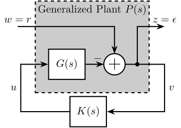
Figure 23: Generalized Plant
The trick is to include a weighting function \(W_S(s)\) in the generalized plant as shown in Figure 24.
Now, the closed-loop transfer function from \(w\) to \(z\) is equal to \(W_s(s)S(s)\) and applying the \(\mathcal{H}_\infty\) synthesis to the weighted generalized plant \(\tilde{P}(s)\) will generate a controller \(K(s)\) such that \(\|W_s(s)S(s)\|_\infty\) is minimized.
Let’s now show how this is equivalent as shaping the sensitivity function:
\begin{align} & \left\| W_s(s) S(s) \right\|_\infty < 1\nonumber \\ \Leftrightarrow & \left| W_s(j\omega) S(j\omega) \right| < 1 \quad \forall \omega\nonumber \\ \Leftrightarrow & \left| S(j\omega) \right| < \frac{1}{\left| W_s(j\omega) \right|} \quad \forall \omega \label{eq:sensitivity_shaping} \end{align}As shown in Equation \eqref{eq:sensitivity_shaping}, the objective of the \(\mathcal{H}_\infty\) synthesis applied on the weighted plant is to make the norm sensitivity function smaller than the inverse of the norm of the weighting function, and that at all frequencies.
Therefore, the choice of the weighting function \(W_s(s)\) is very important: its inverse magnitude will define the wanted upper bound of the sensitivity function magnitude over all frequencies.
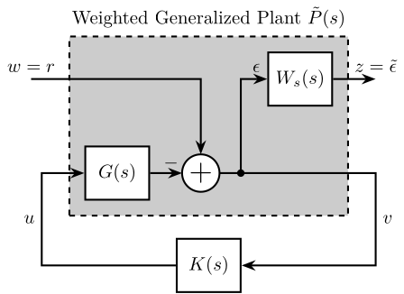
Figure 24: Weighted Generalized Plant
Using matlab, compute the weighted generalized plant shown in Figure 25 as a function of \(G(s)\) and \(W_S(s)\).
Hint
The weighted generalized plant can be defined in Matlab using two techniques:
- by writing manually the 4 transfer functions from \([w, u]\) to \([\tilde{\epsilon}, v]\)
- by pre-multiplying the (non-weighted) generalized plant by a block-diagonal transfer function matrix containing the weights for the outputs \(z\) and
1for the outputs \(v\)
Answer
The two solutions below can be used.
Pw = [Ws -Ws*G;
      1  -G];
The second solution is however more general, and can also be used when weights are added at the inputs by post-multiplying instead of pre-multiplying.
P = [1 -G;
     1 -G];
Pw = blkdiag(Ws, 1)*P;
5.2 Design of Weighting Functions
Weighting function included in the generalized plant must be proper, stable and minimum phase transfer functions.
- proper
- more poles than zeros, this implies \(\lim_{\omega \to \infty} |W(j\omega)| < \infty\)
- stable
- no poles in the right half plane
- minimum phase
- no zeros in the right half plane
Good guidelines for design of weighting function are given in [2].
There is a Matlab function called makeweight that allows to design first-order weights by specifying the low frequency gain, high frequency gain, and the gain at a specific frequency:
W = makeweight(dcgain,[freq,mag],hfgain)
with:
dcgain: low frequency gain[freq,mag]: frequencyfreqat which the gain ismaghfgain: high frequency gain
The Matlab code below produces a weighting function with the following characteristics (Figure 25):
- Low frequency gain of 100
- Gain of 1 at 10Hz
- High frequency gain of 0.5
Ws = makeweight(1e2, [2*pi*10, 1], 1/2);
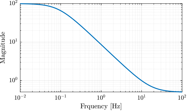
Figure 25: Obtained Magnitude of the Weighting Function
Quite often, higher orders weights are required.
In such case, the following formula can be used:
\begin{equation} W(s) = \left( \frac{ \frac{1}{\omega_0} \sqrt{\frac{1 - \left(\frac{G_0}{G_c}\right)^{\frac{2}{n}}}{1 - \left(\frac{G_c}{G_\infty}\right)^{\frac{2}{n}}}} s + \left(\frac{G_0}{G_c}\right)^{\frac{1}{n}} }{ \left(\frac{1}{G_\infty}\right)^{\frac{1}{n}} \frac{1}{\omega_0} \sqrt{\frac{1 - \left(\frac{G_0}{G_c}\right)^{\frac{2}{n}}}{1 - \left(\frac{G_c}{G_\infty}\right)^{\frac{2}{n}}}} s + \left(\frac{1}{G_c}\right)^{\frac{1}{n}} }\right)^n \label{eq:weight_formula_advanced} \end{equation}The parameters permit to specify:
- the low frequency gain: \(G_0 = lim_{\omega \to 0} |W(j\omega)|\)
- the high frequency gain: \(G_\infty = lim_{\omega \to \infty} |W(j\omega)|\)
- the absolute gain at \(\omega_0\): \(G_c = |W(j\omega_0)|\)
- the absolute slope between high and low frequency: \(n\)
A Matlab function implementing Equation \eqref{eq:weight_formula_advanced} is shown below:
function [W] = generateWeight(args)
    arguments
        args.G0 (1,1) double {mustBeNumeric, mustBePositive} = 0.1
        args.G1 (1,1) double {mustBeNumeric, mustBePositive} = 10
        args.Gc (1,1) double {mustBeNumeric, mustBePositive} = 1
        args.wc (1,1) double {mustBeNumeric, mustBePositive} = 2*pi
        args.n  (1,1) double {mustBeInteger, mustBePositive} = 1
    end

    if (args.Gc <= args.G0 && args.Gc <= args.G1) || (args.Gc >= args.G0 && args.Gc >= args.G1)
        eid = 'value:range';
        msg = 'Gc must be between G0 and G1';
        throwAsCaller(MException(eid,msg))
    end

    s = zpk('s');

    W = (((1/args.wc) * sqrt((1-(args.G0/args.Gc)^(2/args.n))/(1-(args.Gc/args.G1)^(2/args.n)))*s + (args.G0/args.Gc)^(1/args.n)) / ((1/args.G1)^(1/args.n) * (1/args.wc) * sqrt((1-(args.G0/args.Gc)^(2/args.n))/(1-(args.Gc/args.G1)^(2/args.n)))*s + (1/args.Gc)^(1/args.n)))^args.n;

end
Let’s use this function to generate three weights with the same high and low frequency gains, but but different slopes.
W1 = generateWeight('G0', 1e2, 'G1', 1/2, 'Gc', 1, 'wc', 2*pi*10, 'n', 1);
W2 = generateWeight('G0', 1e2, 'G1', 1/2, 'Gc', 1, 'wc', 2*pi*10, 'n', 2);
W3 = generateWeight('G0', 1e2, 'G1', 1/2, 'Gc', 1, 'wc', 2*pi*10, 'n', 3);
The obtained shapes are shown in Figure 26.
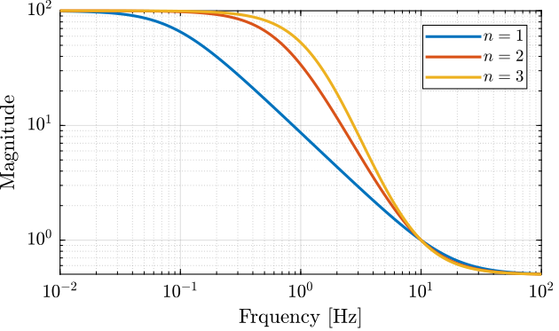
Figure 26: Higher order weights using Equation \eqref{eq:weight_formula_advanced}
5.3 Shaping the Sensitivity Function
Let’s design a controller using the \(\mathcal{H}_\infty\) shaping of the sensitivity function that fulfils the following requirements:
- Bandwidth of at least 10Hz
- Small static errors for step responses
- Robustness: Large module margin \(\Delta M > 0.5\) (\(\Rightarrow \Delta G > 2\) and \(\Delta \phi > 29^o\))
As usual, the plant used is the one presented in Section 1.3.
Translate the requirements as upper bounds on the Sensitivity function and design the corresponding weighting functions using Matlab.
Hint
The typical wanted upper bound of the sensitivity function is shown in Figure 27.
More precisely:
- Recall that the closed-loop bandwidth is defined as the frequency \(|S(j\omega)|\) first crosses \(1/\sqrt{2} = -3dB\) from below
- For the small static error, -60dB is usually enough as other factors (measurement noise, disturbances) will anyhow limit the performances
- Recall that the module margin is equal to the inverse of the \(\mathcal{H}_\infty\) norm of the sensitivity function: \[ \Delta M = \frac{1}{\|S\|_\infty} \]
Remember that the wanted upper bound of the sensitivity function is defined by the inverse magnitude of the weight.
Figure 27: Typical wanted shape of the Sensitivity transfer function
Answer
We want to design the weighting function \(W_s(s)\) such that:
- \(|W_s(j \cdot 2 \pi 10)| = \sqrt{2}\)
- \(|W_s(j \cdot 0)| = 10^3\)
- \(\|W_s\|_\infty = 0.5\)
Using Matlab, such weighting function can be generated using the makeweight function as shown below:
Ws = makeweight(1e3, [2*pi*10, sqrt(2)], 1/2);
Or using the generateWeight function:
Ws = generateWeight('G0', 1e3, ...
                    'G1', 1/2, ...
                    'Gc', sqrt(2), 'wc', 2*pi*10, ...
                    'n', 2);
Let’s say we came up with the following weighting function:
Ws = generateWeight('G0', 1e3, ...
                    'G1', 1/2, ...
                    'Gc', sqrt(2), 'wc', 2*pi*10, ...
                    'n', 2);
The weighting function is then added to the generalized plant.
P = [1 -G;
     1 -G];
Pw = blkdiag(Ws, 1)*P;
And the \(\mathcal{H}_\infty\) synthesis is performed on the weighted generalized plant.
K = hinfsyn(Pw, 1, 1, 'Display', 'on');
Test bounds:  0.5 <=  gamma  <=  0.51

 gamma        X>=0        Y>=0       rho(XY)<1    p/f
5.05e-01     0.0e+00     0.0e+00     3.000e-16     p
Limiting gains...
5.05e-01     0.0e+00     0.0e+00     3.461e-16     p
5.05e-01    -3.5e+01 #  -4.9e-14     1.732e-26     f

Best performance (actual): 0.503
\(\gamma \approx 0.5\) means that the \(\mathcal{H}_\infty\) synthesis generated a controller \(K(s)\) that stabilizes the closed-loop system, and such that the \(\mathcal{H}_\infty\) norm of the closed-loop transfer function from \(w\) to \(z\) is less than \(\gamma\):
\begin{align*} & \| W_s(s) S(s) \|_\infty \approx 0.5 \\ & \Leftrightarrow |S(j\omega)| < \frac{0.5}{|W_s(j\omega)|} \quad \forall \omega \end{align*}This is indeed what we can see by comparing \(|S|\) and \(|W_S|\) in Figure 28.
Obtaining \(\gamma < 1\) means that the \(\mathcal{H}_\infty\) synthesis found a controller such that the specified closed-loop transfer functions are bellow the specified upper bounds.
Yet, obtaining a \(\gamma\) slightly above one does not necessary means the synthesis is unsuccessful. It just means that at some frequency, one of the closed-loop transfer functions is above the specified upper bound by a factor \(\gamma\).
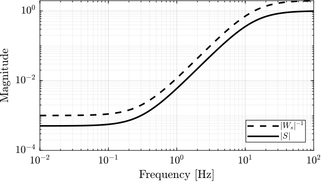
Figure 28: Weighting function and obtained closed-loop sensitivity
5.4 Shaping multiple closed-loop transfer functions - Limitations
As was shown in Section 4, each of the four main closed-loop transfer functions (called the gang of four) will impact different characteristics of the closed-loop system. This is summarized in Table 9.
Therefore, we might want to shape multiple closed-loop transfer functions at the same time. For instance \(S\) could be shape to have good step responses, \(KS\) to limit the input usage and \(T\) to filter measurement noise. When multiple closed-loop transfer function are shaped at the same time, it is refereed to as Mixed-Sensitivity \(\mathcal{H}_\infty\) Control and is the subject of Section 6.
| Specifications | TF | Wanted shape |
|---|---|---|
| Fast Reference Tracking | \(S\) | Set lower bound on the bandwidth |
| Small Steady State Errors | \(S\) | Small low frequency gain |
| Follow Step ref. inputs | \(S\) | Slope of +20dB/dec at low frequency |
| Follow Ramp ref. inputs | \(S\) | Slope of +40dB/dec at low frequency |
| Follow Sin. ref. inputs | \(S\) | Small magnitude centered on the sin. frequency |
| Output Disturbance Rejection | \(S\) | Small gain in the disturbance bandwidth |
| Input Disturbance Rejection | \(GS\) | Small gain in the disturbance bandwidth |
| Prevent notching resonances | \(GS\) | Limit gain around resonance |
| Small Command Amplitude | \(KS\) | Small at high frequency |
| Limitation of the Bandwidth | \(T\) | Set an upper bound on the bandwidth |
| Measurement Noise Filtering | \(T\) | Small high frequency gain |
| Stability margins | \(S\) | Module margin: \(\Vert S\Vert_\infty\) small |
| Robust to unmodelled dynamics | \(T\) | Small at freq. where uncertainty is large |
Depending on which closed-loop transfer function are to be shaped, different weighted generalized plant can be used. Some of them are described below for reference, it is a good exercise to try to re-design such weighted generalized plants.
Shaping of S and KS
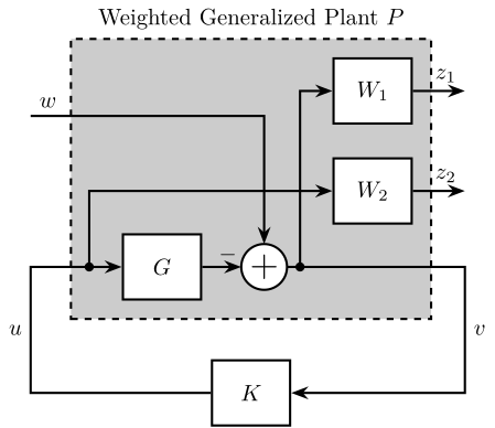
Figure 29: Generalized Plant to shape \(S\) and \(KS\)
Weighting functions:
- \(W_1(s)\) is used to shape \(S\)
- \(W_2(s)\) is used to shape \(KS\)
P = [1 -G
     0  1
     1 -G];
Pw = blkdiag(W1, W2, 1)*P;
Shaping of S and T
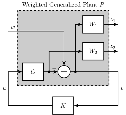
Figure 30: Generalized Plant to shape \(S\) and \(T\)
Weighting functions:
- \(W_1\) is used to shape \(S\)
- \(W_2\) is used to shape \(T\)
P = [1 -G
     0  G
     1 -G];
Pw = blkdiag(W1, W2, 1)*P;
Shaping of S and GS
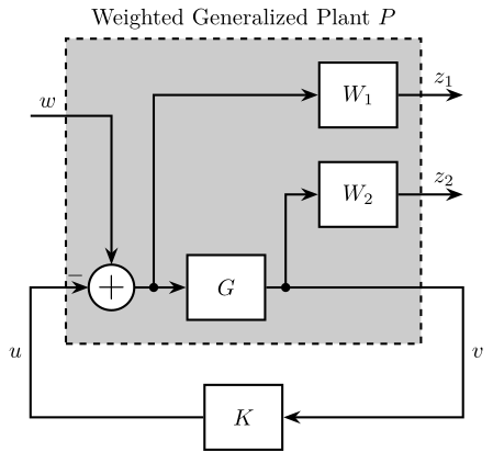
Figure 31: Generalized Plant to shape \(S\) and \(GS\)
Weighting functions:
- \(W_1\) is used to shape \(S\)
- \(W_2\) is used to shape \(GS\)
P = [1 -1
     G -G
     G -G];
Pw = blkdiag(W1, W2, 1)*P;
Shaping of S, T and KS
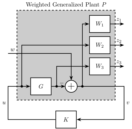
Figure 32: Generalized Plant to shape \(S\), \(T\) and \(KS\)
Weighting functions:
- \(W_1\) is used to shape \(S\)
- \(W_2\) is used to shape \(KS\)
- \(W_3\) is used to shape \(T\)
P = [1 -G
     0  1
     0  G
     1 -G];
Pw = blkdiag(W1, W2, W3, 1)*P;
Shaping of S, T and GS
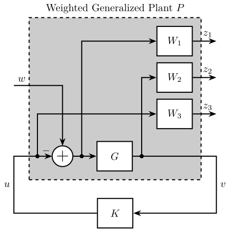
Figure 33: Generalized Plant to shape \(S\), \(T\) and \(GS\)
Weighting functions:
- \(W_1\) is used to shape \(S\)
- \(W_2\) is used to shape \(GS\)
- \(W_3\) is used to shape \(T\)
P = [1 -1
     G -G
     0  1
     G -G];
Pw = blkdiag(W1, W2, W3, 1)*P;
Shaping of S, T, KS and GS
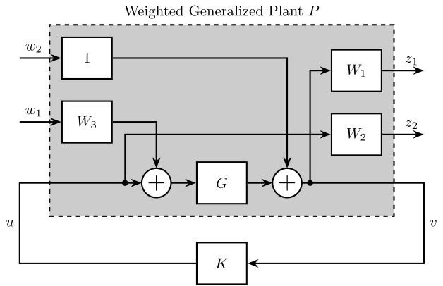
Figure 34: Generalized Plant to shape \(S\), \(T\), \(KS\) and \(GS\)
Weighting functions:
- \(W_1\) is used to shape \(S\)
- \(W_2\) is used to shape \(KS\)
- \(W_1W_3\) is used to shape \(GS\)
- \(W_2W_3\) is used to shape \(T\)
P = [ 1 -G -G
      0  0  1
      1 -G -G];
Pw = blkdiag(W1, W2, 1)*P*blkdiag(1, W3, 1);
When shaping multiple closed-loop transfer functions, one should be very careful about the three following points that are further discussed:
- The shaped closed-loop transfer functions are linked by mathematical relations and cannot be shaped independently
- Closed-loop transfer function can only be shaped in certain frequency range
- The size of the obtained controller may be very large and not implementable in practice
Mathematical relations are linking the closed-loop transfer functions. For instance, the sensitivity function \(S(s)\) and the complementary sensitivity function \(T(s)\) are linked by the following well known relation:
\begin{equation} S(s) + T(s) = 1 \end{equation}This means that \(|S(j\omega)|\) and \(|T(j\omega)|\) cannot be made small at the same time!
It is therefore not possible to shape the four closed-loop transfer functions independently. The weighting function should be carefully design such as these fundamental relations are not violated.
For practical control systems, above some frequency (the control bandwidth), the loop gain is much smaller than 1. On the other size, there is a frequency range where the loop gain is much larger than 1, this frequency range is called the bandwidth. Let’s see what does that means for the closed-loop transfer function. First, take the case of the sensibility function:
\begin{align*} &|G(j\omega) K(j\omega)| \ll 1 \Longrightarrow |S(j\omega)| = \frac{1}{1 + |G(j\omega)K(j\omega)|} \approx 1 \\ &|G(j\omega) K(j\omega)| \gg 1 \Longrightarrow |S(j\omega)| = \frac{1}{1 + |G(j\omega)K(j\omega)|} \approx \frac{1}{|G(j\omega)K(j\omega)|} \end{align*}This means that the Sensitivity function cannot be shaped at frequencies where the loop gain is small.
Similar relationship can be found for \(T\), \(KS\) and \(GS\).
Determine the approximate norms of \(T\), \(KS\) and \(GS\) for large loop gains (\(|G(j\omega) K(j\omega)| \gg 1\)) and small loop gains (\(|G(j\omega) K(j\omega)| \ll 1\)).
Hint
You can follows this procedure for \(T\), \(KS\) and \(GS\):
- Write the closed-loop transfer function as a function of \(K(s)\) and \(G(s)\)
- Take \(|K(j\omega)G(j\omega)| \gg 1\) and conclude on the norm of the closed-loop transfer function
- Take \(|K(j\omega)G(j\omega)| \ll 1\) and conclude
Answer
The obtained constrains are shown in Figure 35.
Depending on the frequency band, the norms of the closed-loop transfer functions are a function of the controller \(K\) and therefore can be shaped. However, in some frequency band, the norms do not depend on the controller and therefore cannot be shaped.
Therefore the weighting functions should only focus on certainty frequency range depending on the transfer function being shaped. These regions are summarized in Figure 35.
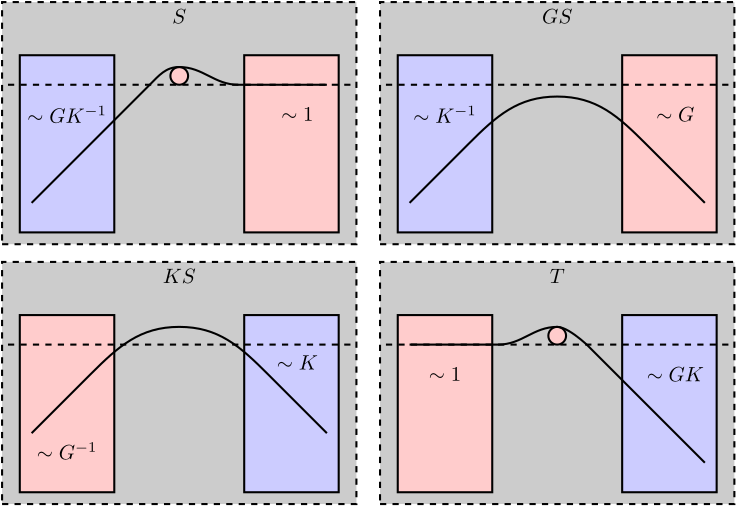
Figure 35: Shaping the Gang of Four. Blue regions indicate that the transfer function can be shaped using \(K\). Red regions indicate this is not the case
The order (e.g. number of state) of the controller given by the \(\mathcal{H}_\infty\) synthesis is equal to the order (e.g. number of state) of the weighted generalized plant. It is thus equal to the sum of the number of state of the non-weighted generalized plant and the number of state of all the weighting functions. Then, the \(\mathcal{H}_\infty\) synthesis usually generate a controller with a very high order that is not implementable in practice.
Two approaches can be used to obtain controllers with reasonable order:
- use simple weights (usually first order)
- perform a model reduction on the obtained high order controller
6 Mixed-Sensitivity \(\mathcal{H}_\infty\) Control - Example
Let’s now apply the \(\mathcal{H}_\infty\) Shaping control procedure on a practical example.
In Section 6.1 the control problem is presented. The design procedure used to apply the \(\mathcal{H}_\infty\) Mixed Sensitivity synthesis is described in Section 6.2.
The important step of interpreting the specifications as wanted shape of closed-loop transfer functions is performed in Section 6.3.
Finally, the shaping of closed-loop transfer functions is performed in Sections 6.4, 6.5 and 6.6.
6.1 Control Problem
Let’s consider our usual test system shown in Figure 36.
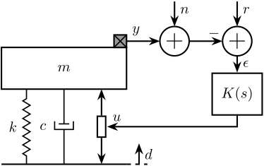
Figure 36: Test System consisting of a payload with a mass \(m\) on top of an active system with a stiffness \(k\), damping \(c\) and an actuator. A feedback controller \(K(s)\) is added to position / isolate the payload.
The control specifications are:
- The displacement \(y\) should follow reference inputs \(r\) with negligible static error after 0.1s
- Reject disturbances \(d\) in less than 0.1s
- Limit the effect of measurement noise \(n\) on the output displacement \(y\)
- Obtain a Robust System with good stability margins
The considered inputs are:
- disturbances \(d\) as step inputs with an amplitude of \(5\,\mu m\)
- reference inputs with are ramp inputs with a slope of \(100\,\mu m/s\) and a time duration of \(0.2\,s\)
- measurement noise \(n\) with a large spectral density at high frequency (increasing starting from 100Hz)
6.2 Control Design Procedure
Here is the general design procedure that will be followed:
- Compute the model of the plant
- Write the control system as a general control problem
- Translate the specifications into the wanted shape of closed-loop transfer functions
- Chose the suitable weighted general plant to shape the wanted quantities
- Shape sequentially the chosen closed-loop transfer functions
Let’s first convert the system of Figure 36 into the classical feedback architecture of Figure 37.
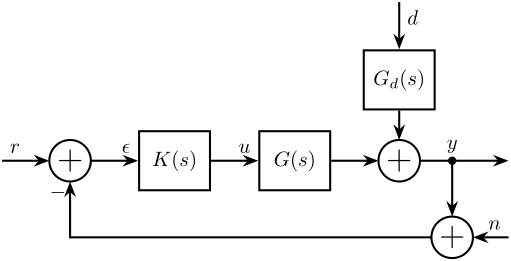
Figure 37: Block diagram corresponding to the example system
The two transfer functions present in the system are derived and defined below:
1: k = 1e6; % Stiffness [N/m]
2: c = 4e2; % Damping [N/(m/s)]
3: m = 10; % Mass [kg]
4:
5: % Control Plant
6: G = 1/(m*s^2 + c*s + k);
7: % Disturbance dynamics
8: Gd = (c*s + k)/(m*s^2 + c*s + k);
We also define the inputs signals that will be used for time domain simulations. They are graphically shown in Figure 38.
 9: % Time Vector
10: t = 0:1e-4:0.5;
11:
12: % Reference Input
13: r = zeros(size(t));
14: r(t>0.05 & t<=0.25) = 1e-4*(t(t>0.05 & t<=0.25)-0.05);
15: r(t>0.25) = 2e-5;
16:
17: % Measurement Noise
18: Fs = 1e3; % Sampling Frequency [Hz]
19: Ts = 1/Fs; % Sampling Time [s]
20: n = sqrt(Fs/2)*randn(1, length(t)); % Signal with an ASD equal to one
21: n = lsim(1e-6*(s + 2*pi*1e2)^2/(s + 2*pi*1e3)^2/(1+s/2/pi/500), n, t)'; % Shaped noise
22:
23: % Disturbance
24: d = zeros(size(t));
25: d(t>0.3) = 5e-6;
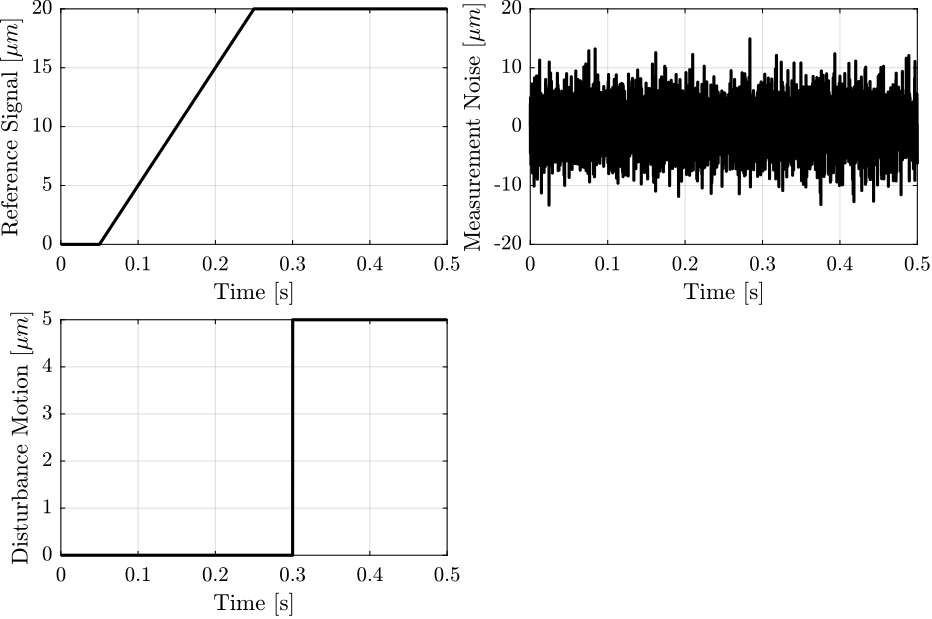
Figure 38: Time domain inputs signals
We also define the generalized plant corresponding to the system and that will be used for time domain simulations (Figure 39).
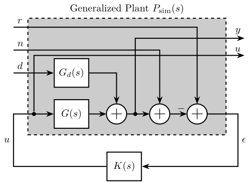
Figure 39: Generalized plant that will be used for simulations
The Generalized plant of Figure 39 is defined on Matlab as follows:
26: Psim = [0  0  Gd  G
27:         0  0  0   1
28:         1 -1 -Gd -G];
29:
30: Psim.InputName = {'r', 'n', 'd', 'u'};
31: Psim.OutputName = {'y', 'u', 'e'};
Time domain simulations will be performed by first computing the closed-loop system using the lft command and then using the lsim command on the closed-loop system:
32: % Compute the closed-Loop System, K is the controller
33: P_CL = lft(Psim, K);
34:
35: % Time simulation of the closed-loop system with specified inputs
36: z = lsim(P_CL, [r; n; d], t);
37: % The two outputs are
38: y = z(:,1); % Output Motion [m]
39: u = z(:,2); % Input usage [N]
6.3 Modern Interpretation of control specifications
- Translate the control specifications into wanted shape of closed-loop transfer functions
- Conclude and the closed-loop transfer functions to be shaped
- Chose a general configuration architecture that allows to shape these transfer function
- Using Matlab, define the generalized plant
After converting the control specifications into wanted shape of closed-loop transfer functions, we might come up with the Table 10.
In such case, we want to shape \(S\), \(GS\) and \(T\).
| Specification | TF | Wanted Shape |
|---|---|---|
| Follow Step Reference | \(S\) | +40dB of slope at low frequency |
| Reject Disturbances | \(S\), \(GS\) | Small gain |
| Reject measurement noise | \(T\) | Small high frequency (>100Hz) gain |
| Robust System | \(S\) | Small \(\Vert S \Vert_\infty\) |
To do so, we use to generalized plant shown in Figure 40 for the synthesis where the three closed-loop tranfert functions from \(w\) to \([z_1\,,z_2\,,z_3]\) are respectively \(S\), \(GS\) and \(T\).
This generalized plant is defined on Matlab as follows:
40: P = [1 -1
41:      G -G
42:      0  1
43:      G -G];
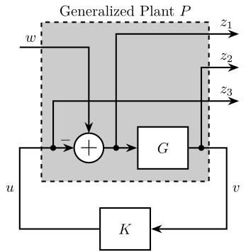
Figure 40: Generalized plant chosen for the shaping of \(S\), \(GS\) \(T\)
However, to performed the \(\mathcal{H}_\infty\) loop shaping, we have to include weighting function to the Generalized plant. We obtain the weighted generalized plant in Figure 41, and that is computed using Matlab as follows:
44: Pw = blkdiag(W1, W2, W3, 1)*P;
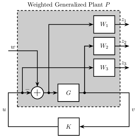
Figure 41: Generalized weighted plant used for the \(\mathcal{H}_\infty\) Synthesis
Finlay, performing the \(\mathcal{H}_\infty\) Shaping of \(S\), \(GS\) and \(T\) is as simple as ruining the hinfsyn command:
45: K = hinfsyn(Pw, 1, 1);
Now let’s shape the three closed-loop transfer functions sequentially:
6.4 Step 1 - Shaping of \(S\)
Let’s first shape the Sensitivity function as it is usually the most important of the Gang of four closed-loop transfer functions. To do so, we have to create a weight \(W_1(s)\) that defines the wanted upper bound on \(|S(j\omega)|\):
- small low frequency gain: \(|S(j\cdot 0)| = 10^{-3}\)
- minimum crossover frequency of \(\approx 10Hz\): \(|S(j2\pi 10)| < \frac{1}{\sqrt{2}}\)
- small maximum peak magnitude for robustness properties: \(\|S\|_\infty < 2\)
The weighting function is design using the generateWeigh function and its inverse shape can be seen in Figure
46: W1 = generateWeight('G0', 1e3, ...
47:                     'G1', 1/2, ...
48:                     'Gc', sqrt(2), 'wc', 2*pi*10, ...
49:                     'n', 1);
To not constrain \(GS\) and \(T\) for the shaping of \(S\), \(W_2\) and \(W_3\) are first taken as very small gains:
50: W2 = tf(1e-8);
51: W3 = tf(1e-8);
The \(\mathcal{H}_\infty\) synthesis is performed and the obtained closed-loop transfer functions \(S\), \(GS\), and \(T\) and compared with the upper bounds set by the weighting functions in Figure 42.
52: Pw = blkdiag(W1, W2, W3, 1)*P;
53: K1 = hinfsyn(Pw, 1, 1, 'Display', 'on');
Test bounds:  0.5 <=  gamma  <=  0.51

 gamma        X>=0        Y>=0       rho(XY)<1    p/f
5.05e-01     0.0e+00     0.0e+00     5.511e-14     p
Limiting gains...
5.05e-01     0.0e+00     0.0e+00     1.867e-14     p

Best performance (actual): 0.502
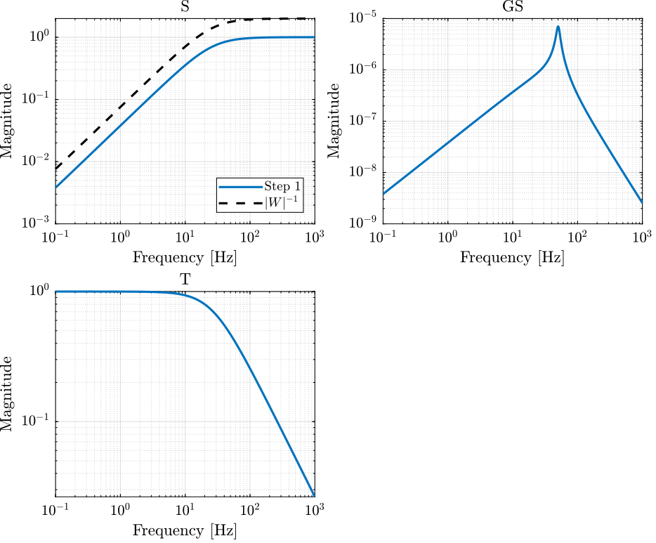
Figure 42: Obtained Shape Closed-Loop transfer functions (dashed black lines indicate inverse magnitude of the weighting functions)
Time domain simulation is then performed and the obtained output displacement and control inputs are shown in Figure 43.
We can see:
- we are not able to follow the ramp input. This have to be solved by modifying the weighting function \(W_1(s)\)
- we have poor rejection of disturbances. This we be solve by shaping \(GS\) in Section 6.5
- we have quite large effect of the measurement noise. This will be solved by shaping \(T\) in Section 6.6
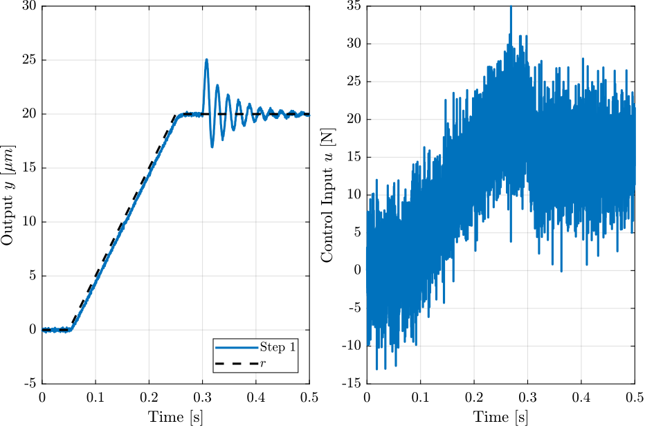
Figure 43: Time domain simulation results
Remember that in order to follow ramp inputs, the sensitivity function should have a slope of +40dB/dec at low frequency (Table 9).
To do so, let’s modify \(W_1\) to impose a slope of +40dB/dec at low frequency. This can simple be done by using a second order weight:
54: W1 = generateWeight('G0', 1e3, ...
55:                     'G1', 1/2, ...
56:                     'Gc', sqrt(2), 'wc', 2*pi*15, ...
57:                     'n', 2);
The \(\mathcal{H}_\infty\) synthesis is performed using the new weights and the obtained closed-loop shaped are shown in figure 44.
The time domain signals are shown in Figure 45 and it is confirmed that the ramps are now follows without static errors.
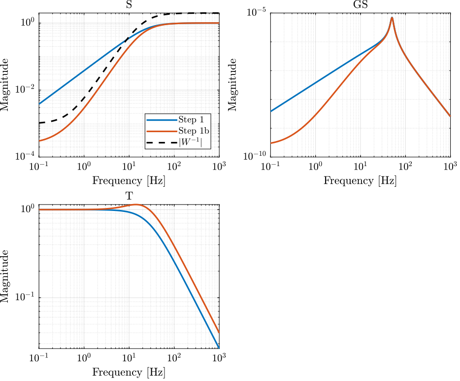
Figure 44: Obtained Shape Closed-Loop transfer functions
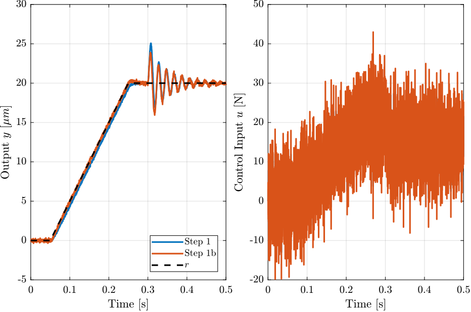
Figure 45: Time domain simulation results
6.5 Step 2 - Shaping of \(GS\)
Looking at Figure 46, it is clear that the rejection of disturbances is not satisfactory. This can also be seen by the large peak of \(GS\) in Figure 44.
This poor rejection of disturbances is actually due to the fact that the obtain controller has at notch at the resonance frequency of the plant.
To overcome this issue, we can simply increase the magnitude of \(W_2\) to limit the peak magnitude of \(GS\) Let’s take \(W_2\) as a simple constant gain:
58: W2 = tf(4e5);
The \(\mathcal{H}_\infty\) Synthesis is performed and the obtained closed-loop transfer functions are shown in Figure 46.
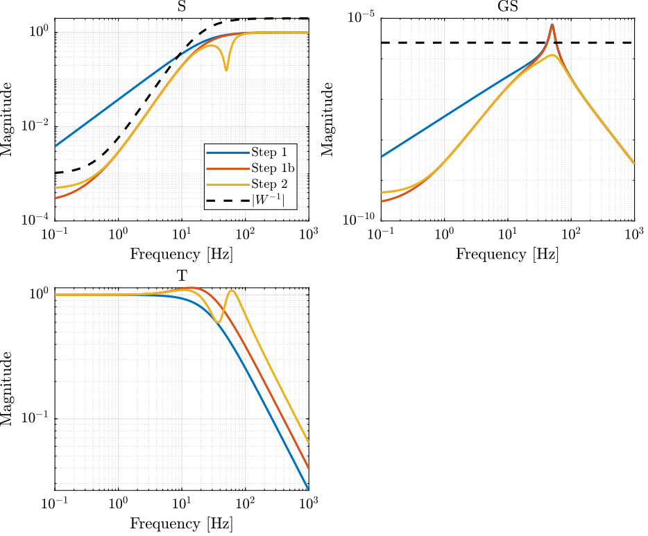
Figure 46: Obtained Shape Closed-Loop transfer functions
Time domain simulation results are shown in Figure 47. If is shown that indeed, the disturbance rejection performance are much better and only very small oscillation is obtained.
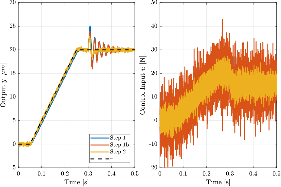
Figure 47: Time domain simulation results
6.6 Step 3 - Shaping of \(T\)
Finally, we want to limit the effect of the noise on the displacement output.
To do so, \(T\) is shaped such that its high frequency gain is reduced.
This is done by increasing the high frequency gain of the weighting function \(W_3\) until the \(\mathcal{H}_\infty\) synthesis gives \(\gamma \approx 1\).
The final weighting function \(W_3\) is defined as follows:
59: W3 = generateWeight('G0', 1e-1, ...
60:                     'G1', 1e4, ...
61:                     'Gc', 1, 'wc', 2*pi*70, ...
62:                     'n', 2);
The \(\mathcal{H}_\infty\) synthesis is performed and \(\gamma\) is closed to one. The obtained closed-loop transfer functions are shown in Figure 48 and we can obverse that:
- The high frequency gain of \(T\) is indeed reduced
- This comes as the expense of a large magnitude both \(GS\) and \(S\). This means we will probably have slightly less good disturbance rejection and tracking performances.
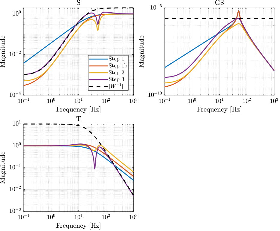
Figure 48: Obtained Shape Closed-Loop transfer functions
The time domain simulation signals are shown in Figure 49. We can indeed see a slightly less good disturbance rejection. However, the vibrations induced by the sensor noise is well reduced. This can be seen when zooming on the output signal in Figure 50.
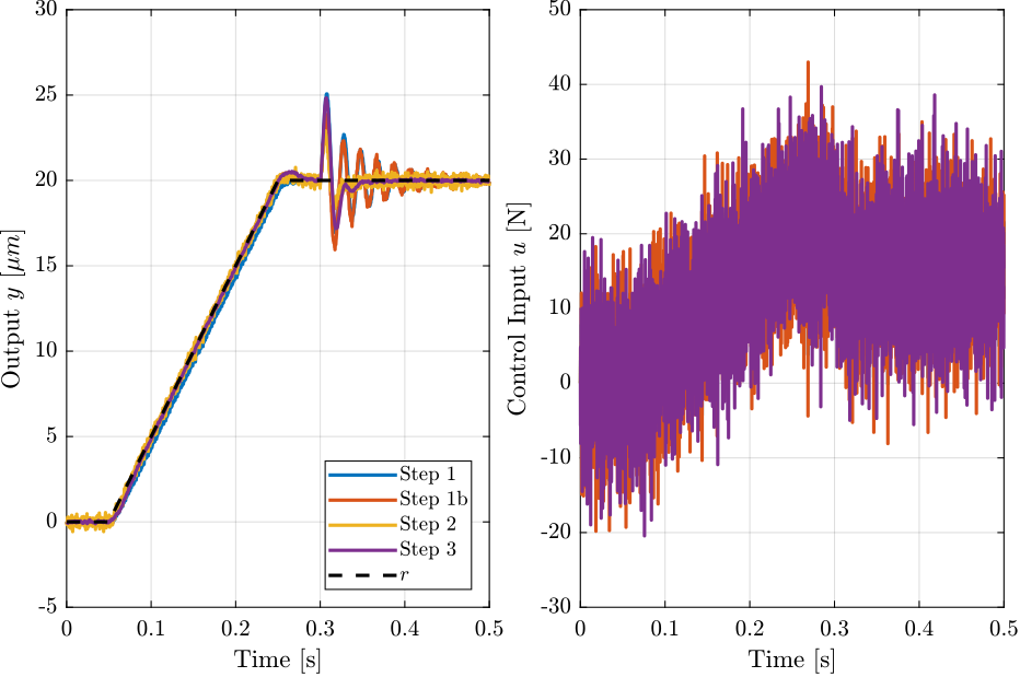
Figure 49: Time domain simulation results
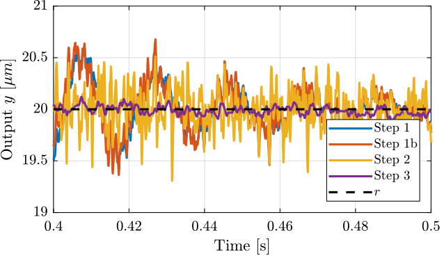
Figure 50: Zoom on the output signal
6.7 Conclusion and Discussion
Hopefully this practical example will help you apply the \(\mathcal{H}_\infty\) Shaping synthesis on other control problems.
As an exercise, plot and analyze the evolution of the controller and loop gain transfer functions during the 3 synthesis steps.
If the large input usage is considered to be not acceptable, the shaping of \(KS\) could be included in the synthesis and all the Gang of four closed-loop transfer function shapes.
7 Conclusion
Hopefully, this document gave you a glimpse on how useful and powerful the \(\mathcal{H}_\infty\) loop shaping synthesis can be. One of the true power of \(\mathcal{H}_\infty\) synthesis is that is can easily be applied to multi-input multi-output systems! If you want to know more about the “\(\mathcal{H}_\infty\) and robust control world” some resources are given below.
Resources
For a complete treatment of multivariable robust control, I would highly recommend this book [3]. If you want to nice reference book in French, look at [4].
You can also look at the very good lectures below.