Bank of Linear Filters - Matlab

Table of ContentsClose

1 Low Pass

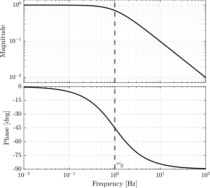
1.1 First Order Low Pass Filter

$H (s) = \frac{1}{1 + s / ω_{0}}$

Parameters:

$ω_{0}$ : cut-off frequency in [rad/s]

Characteristics:

Low frequency gain of $1$
Roll-off equals to -20 dB/dec

Matlab code:

Copy
w0 = 2*pi; % Cut-off Frequency [rad/s]

H = 1/(1 + s/w0);

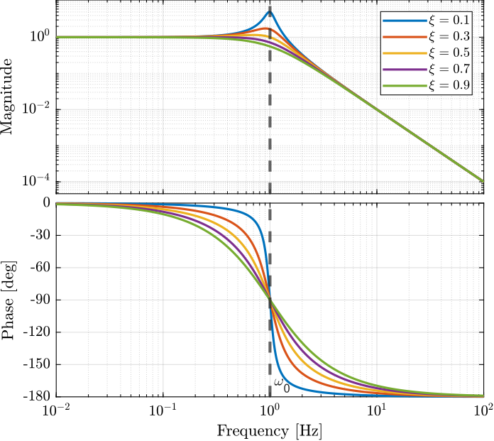
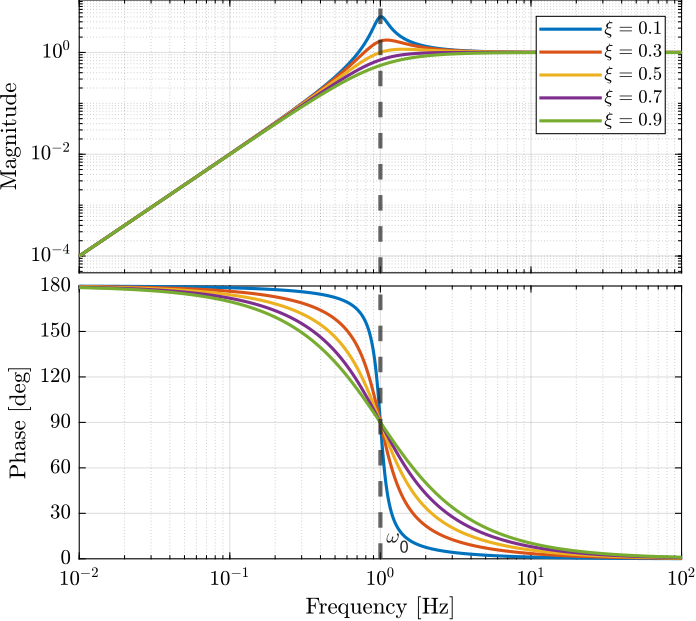
1.2 Second Order

$H (s) = \frac{1}{1 + 2 ξ / ω_{0} s + s^{2} / ω_{0}^{2}}$

Parameters:

$ω_{0}$ :
$ξ$ : Damping ratio

Characteristics:

Low frequency gain: 1
High frequency roll off: - 40 dB/dec

Matlab code:

Copy
w0 = 2*pi; % Cut-off frequency [rad/s]
xi = 0.3; % Damping Ratio

H = 1/(1 + 2*xi/w0*s + s^2/w0^2);

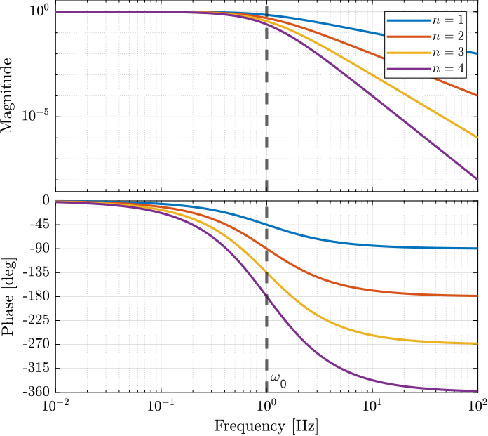
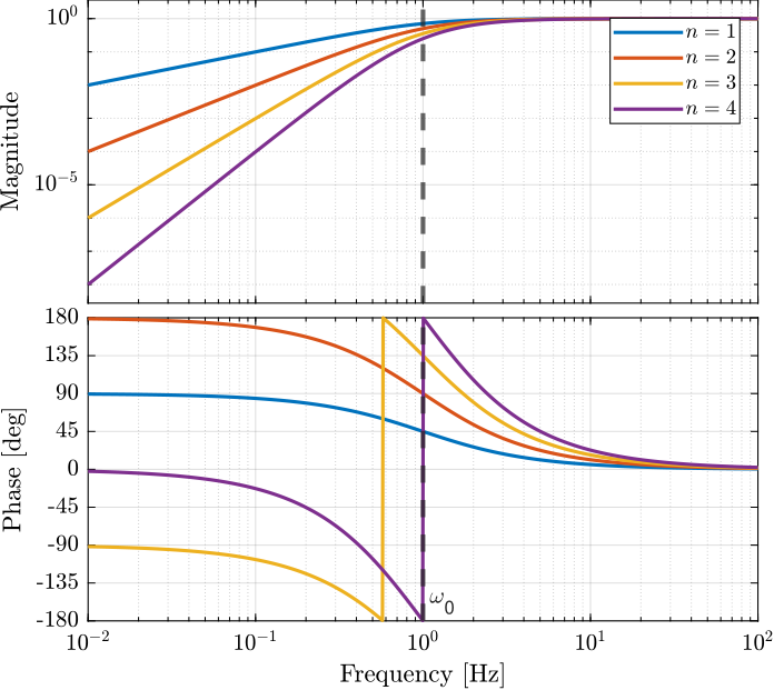
1.3 Combine multiple first order filters

$H (s) = {(\frac{1}{1 + s / ω_{0}})}^{n}$

Matlab code:

Copy
w0 = 2*pi; % Cut-off frequency [rad/s]
n = 3; % Filter order

H = (1/(1 + s/w0))^n;

2 High Pass

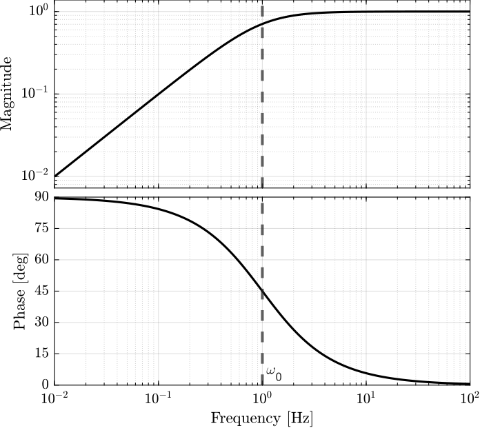
2.1 First Order

$H (s) = \frac{s / ω_{0}}{1 + s / ω_{0}}$

Parameters:

$ω_{0}$ : cut-off frequency in [rad/s]

Characteristics:

High frequency gain of $1$
Low frequency slow of +20 dB/dec

Matlab code:

Copy
w0 = 2*pi; % Cut-off frequency [rad/s]

H = (s/w0)/(1 + s/w0);

2.2 Second Order

$H (s) = \frac{s^{2} / ω_{0}^{2}}{1 + 2 ξ / ω_{0} s + s^{2} / ω_{0}^{2}}$

Parameters:

$ω_{0}$ :
$ξ$ : Damping ratio

Matlab code:

Copy
w0 = 2*pi; % [rad/s]
xi = 0.3;

H = (s^2/w0^2)/(1 + 2*xi/w0*s + s^2/w0^2);

2.3 Combine multiple filters

$H (s) = {(\frac{s / ω_{0}}{1 + s / ω_{0}})}^{n}$

Matlab code:

Copy
w0 = 2*pi; % [rad/s]
n = 3;

H = ((s/w0)/(1 + s/w0))^n;

3 Band Pass

3.1 Second Order

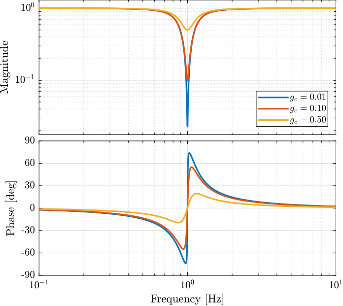
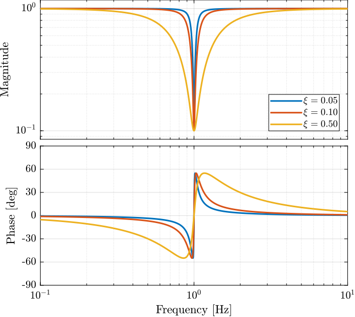
4 Notch

4.1 Second Order

\begin{matrix} (1) & \frac{s^{2} + 2 g_{c} ξ ω_{n} s + ω_{n}^{2}}{s^{2} + 2 ξ ω_{n} s + ω_{n}^{2}} \end{matrix}

Parameters:

$ω_{n}$ : frequency of the notch
$g_{c}$ : gain at the notch frequency
$ξ$ : damping ratio (notch width)

Matlab code:

Copygc = 0.02;
xi = 0.1;
wn = 2*pi;

H = (s^2 + 2*gm*xi*wn*s + wn^2)/(s^2 + 2*xi*wn*s + wn^2);

5 Chebyshev

5.1 Chebyshev Type I

Copy
n = 4; % Order of the filter
Rp = 3; % Maximum peak-to-peak ripple [dB]
Wp = 2*pi; % passband-edge frequency [rad/s]

[A,B,C,D] = cheby1(n, Rp, Wp, 'high', 's');
H = ss(A, B, C, D);

6 Lead - Lag

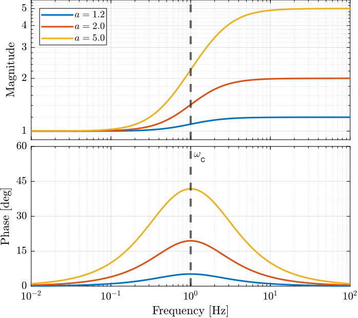
6.1 Lead

\begin{matrix} (2) & H (s) = \frac{1 + \frac{s}{w_{c} / \sqrt{a}}}{1 + \frac{s}{w_{c} \sqrt{a}}}, a > 1 \end{matrix}

Parameters:

$ω_{c}$ : frequency at which the phase lead is maximum
$a$ : parameter to adjust the phase lead, also impacts the high frequency gain

Characteristics:

the low frequency gain is $1$
the high frequency gain is $a$
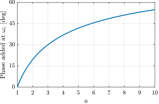
the phase lead at $ω_{c}$ is equal to (Figure 10): $∠ H (j ω_{c}) = \tan^{- 1} (\sqrt{a}) - \tan^{- 1} (1 / \sqrt{a})$

Matlab code:

Copy
a  = 0.6;  % Amount of phase lead / width of the phase lead / high frequency gain
wc = 2*pi; % Frequency with the maximum phase lead [rad/s]

H = (1 + s/(wc/sqrt(a)))/(1 + s/(wc*sqrt(a)));

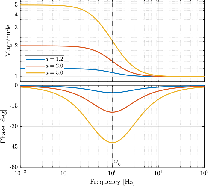
6.2 Lag

\begin{matrix} (3) & H (s) = \frac{w_{c} \sqrt{a} + s}{\frac{w_{c}}{\sqrt{a}} + s}, a > 1 \end{matrix}

Parameters:

$ω_{c}$ : frequency at which the phase lag is maximum
$a$ : parameter to adjust the phase lag, also impacts the low frequency gain

Characteristics:

the low frequency gain is increased by a factor $a$
the high frequency gain is $1$ (unchanged)
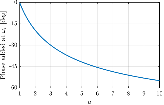
the phase lag at $ω_{c}$ is equal to (Figure 12): $∠ H (j ω_{c}) = \tan^{- 1} (1 / \sqrt{a}) - \tan^{- 1} (\sqrt{a})$

Matlab code:

Copy
a  = 0.6;  % Amount of phase lag / width of the phase lag / high frequency gain
wc = 2*pi; % Frequency with the maximum phase lag [rad/s]

H = (wc*sqrt(a) + s)/(wc/sqrt(a) + s);

7 Complementary

8 Performance Weight

8.1 Nice combination

\begin{matrix} (4) & W (s) = G_{c} * {(\frac{\frac{1}{ω_{0}} \sqrt{\frac{1 - {(\frac{G_{0}}{G_{c}})}^{\frac{2}{n}}}{1 - {(\frac{G_{c}}{G_{\infty}})}^{\frac{2}{n}}}} s + {(\frac{G_{0}}{G_{c}})}^{\frac{1}{n}}}{\frac{1}{ω_{0}} \sqrt{\frac{1 - {(\frac{G_{0}}{G_{c}})}^{\frac{2}{n}}}{{(\frac{G_{\infty}}{G_{c}})}^{\frac{2}{n}} - 1}} s + 1})}^{n} \end{matrix}

Copy
n = 2; w0 = 2*pi*11; G0 = 1/10; G1 = 1000; Gc = 1/2;
wL = Gc*(((G1/Gc)^(1/n)/w0*sqrt((1-(G0/Gc)^(2/n))/((G1/Gc)^(2/n)-1))*s + (G0/Gc)^(1/n))/(1/w0*sqrt((1-(G0/Gc)^(2/n))/((G1/Gc)^(2/n)-1))*s + 1))^n;

n = 3; w0 = 2*pi*9; G0 = 10000; G1 = 0.1; Gc = 1/2;
wH = Gc*(((G1/Gc)^(1/n)/w0*sqrt((1-(G0/Gc)^(2/n))/((G1/Gc)^(2/n)-1))*s + (G0/Gc)^(1/n))/(1/w0*sqrt((1-(G0/Gc)^(2/n))/((G1/Gc)^(2/n)-1))*s + 1))^n;

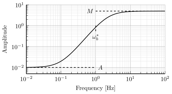
8.2 Alternative

Copy
w0 = 2*pi; % [rad/s]
A = 1e-2;
M = 5;

H = (s/sqrt(M) + w0)^2/(s + w0*sqrt(A))^2;

9 Combine Filters

9.1 Additive

[ ] Explain how phase and magnitude combine

9.2 Multiplicative

10 Filters representing noise

Let’s consider a noise $n$ that is shaped from a white-noise $\tilde{n}$ with unitary PSD ( $Φ_{\tilde{n}} (ω) = 1$ ) using a transfer function $G (s)$ . The PSD of $n$ is then: $Φ_{n} (ω) = | G (j ω) |^{2} Φ_{\tilde{n}} (ω) = | G (j ω) |^{2}$

The PSD $Φ_{n} (ω)$ is expressed in ${unit}^{2} / Hz$ .

And the root mean square (RMS) of $n (t)$ is: $σ_{n} = \sqrt{\int_{0}^{\infty} Φ_{n} (ω) d ω}$

10.1 First Order Low Pass Filter

$G (s) = \frac{g_{0}}{1 + \frac{s}{ω_{c}}}$

Copy
g0 = 1; % Noise Density in unit/sqrt(Hz)
wc = 1; % Cut-Off frequency [rad/s]

G = g0/(1 + s/wc);

% Frequency vector [Hz]
freqs = logspace(-3, 3, 1000);

% PSD of n in [unit^2/Hz]
Phi_n = abs(squeeze(freqresp(G, freqs, 'Hz'))).^2;

% RMS value of n in [unit, rms]
sigma_n = sqrt(trapz(freqs, Phi_n))

$σ = \frac{1}{2} g_{0} \sqrt{ω_{c}}$ with:

$g_{0}$ the Noise Density of $n$ in $unit / \sqrt{H z}$
$ω_{c}$ the bandwidth over which the noise is located, in rad/s
$σ$ the rms noise

If the cut-off frequency is to be expressed in Hz: $σ = \frac{1}{2} g_{0} \sqrt{2 π f_{c}} = \sqrt{\frac{π}{2}} g_{0} \sqrt{f_{c}}$

Thus, if a sensor is said to have a RMS noise of $σ = 10 n m r m s$ over a bandwidth of $ω_{c} = 100 r a d / s$ , we can estimated the noise density of the sensor to be (supposing a first order low pass filter noise shape): $g_{0} = \frac{2 σ}{\sqrt{ω_{c}}} [m / \sqrt{H z}]$

Copy
2*10e-9/sqrt(100)

2e-09

Copy
6*0.5*20e-12*sqrt(2*pi*100)

1.504e-09