EUSPEN
Table of Contents
- 1. Tutorial: Design concepts for sub-micrometer positioning @huub_janssen
- 2. Keynote: Mechatronic challenges in optical lithography @hans_butler
- 2.1. Introduction
- 2.2. Chip manufacturing loop
- 2.3. Imaging process - Basics
- 2.4. From stepper to scanner
- 2.5. Dual stage scanners
- 2.6. Immersion technology
- 2.7. Multiple Patterning
- 2.8. Machine layout
- 2.9. EUV Lithography
- 2.10. The future: high-NA EUV
- 2.11. Challenges for future Optical Lithography machines
- 2.12. Conclusion
- 3. Keynote: High precision mechatronic approaches for advanced nanopositioning and nanomeasuring technologies @eberhard_manske
- 3.1. Coordinate Measurement Machines (CMM)
- 3.2. Difference between CMM and nano-CMM
- 3.3. How to do nano-CMM
- 3.4. Concept - Minimization of the Abbe Error
- 3.5. Minimization of residual Abbe error
- 3.6. Compare of long travel guiding systems
- 3.7. Extended 6 DoF Abbe comparator principle
- 3.8. Practical Realisation
- 3.9. Tilt Compensation
- 3.10. Comparison of long travail guiding systems - Bis
- 3.11. Drive concept
- 3.12. NPMM-200 with extended measuring volume
- 3.13. measurement capability
- 3.14. Extension of the measuring range (700mm)
- 3.15. Inverse kinematic concept - Tetrahedrical concept
- 3.16. Inverse kinematic concept - Scanning probe principle
- 3.17. Inverse kinematic concept - Compact measuring head
- 3.18. Inverse kinematic concept - Scanning probe principle
- 3.19. Conclusion
- 4. Designing anti-aliasing-filters for control loops of mechatronic systems regarding the rejection of aliased resonances @ulrich_schonhoff
- 5. Flexure positioning stage based on delta technology for high precision and dynamic industrial machining applications @mikael_bianchi
- 6. Multivariable performance analysis of position-controlled payloads with flexible eigenmodes @luca_mettenleiter
- 7. High-precision motion system design by topology optimization considering additive manufacturing @arnoud_delissen
- 8. A multivariable experiment design framework for accurate FRF identification of complex systems @nic_dirkx
- 9. Reducing control delay times to enhance dynamic stiffness of magnetic bearings @jan_philipp_schmidtmann
- 10. Digital twins in control: From fault detection to predictive maintenance in precision mechatronics @koen_classens
This report is also available as a pdf.
1 Tutorial: Design concepts for sub-micrometer positioning @huub_janssen
1.1 Positioning Terminology
- Accuracy: Accuracy describes how close the mean result is to the reference value. (Figure 1)
- Repeatability: Repeatability describes the variation between results. (Figure 1)
- Resolution: The resolution of a system is equal to the smallest incremental step that can be made (Figure 2)
- Stability: The stability of a system is the maximum deviation from a constant reference value over time. The stability is always related to the time frame taken into account. (Figure 3)
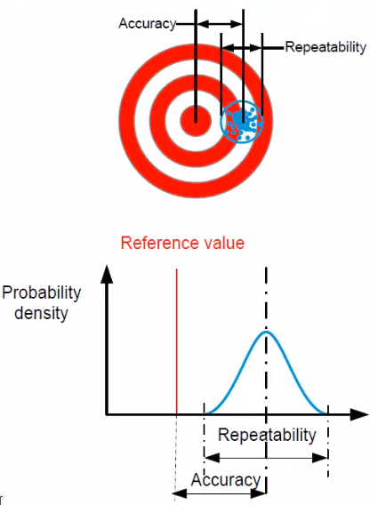
Figure 1: Accuracy and Repeatability
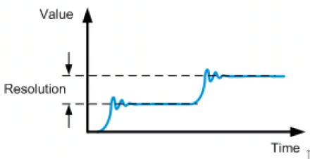
Figure 2: Position Resolution
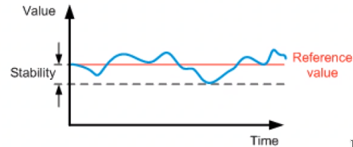
Figure 3: Position Stability
1.2 Principles of accuracy
Limited stiffness, play and friction will induce an hysteresis for a positioning system as shown in Figure 4.
The hysteresis can actually help estimating the play and friction present in the system.
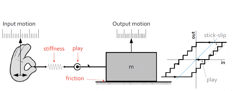
Figure 4: Stiffness, play and Friction
Ways to make the hysteresis smaller:
- avoid play (=> use compliant elements)
- minimize friction
- use high stiffness
The position uncertainty of a system can be estimated as follow (Figure 5):
\begin{equation} \text{Position Uncertainty} = \text{play} + 2 \times \text{Virtual Play} \end{equation}where the virtual play can be estimated as follow:
\begin{equation} \text{Virtual Play} = \frac{\text{Friction Force}}{\text{Actuator Stiffness}} = \frac{F_w}{c} \end{equation}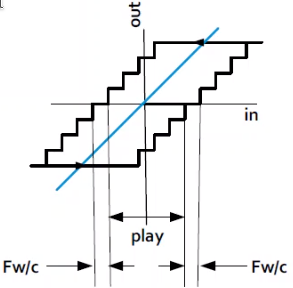
Figure 5: Hysterestis, play and virtual play
When considering dynamics, the goal is to make the first resonance frequency much higher than the frequency of the wanted motion. Thus, the general recommendation is then to minimize mass and to increase stiffness.
Moreover, we generally want things to be predictable:
- constant, preferably no friction. Note that it is very difficult to make a system with constant friction in practice, so better make a system with no friction.
- no play
- high stiffness
- low pass
1.3 Case 1 - Estimate the virtual play
Estimate the virtual play of the system in Figure 6 with following characteristics:
- Payload: \(m = 20\,kg\)
- Friction coefficient in drive direction: \(f = 0.05\)
- Table stroke: \(L = 300\,mm\)
- Screw spindle inner diameter: \(d = 8\, mm\)
- Spindle Material: Stainless steel
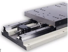
Figure 6: Studied system for “Case 1”
First the friction force can be calculated as the vertical mass times the friction coefficient:
\begin{equation} F_w = (mg) f \end{equation}Then, the axial stiffness of the screw spindle is computed:
\begin{equation} c = \frac{A}{L} E \end{equation}with:
- \(A = \pi d^2\) is the screw section area
- \(L = 300\,mm\) is the screw length
- \(E\) is the Young modulus of stainless steel
And finally:
\begin{equation} \text{Virtual Play} = \frac{F_w}{c} \approx 0.6\,\mu m \end{equation}1.4 Conventional elements for constraining DoFs
There exist many conventional elements for constraining DoFs. Some of them are:
- Struts with ball joint: 1DoF constrained (Figure 7)
- Ball bearing: 5DoF constrained (Figure 8)
- Guide with roller bearing: 4DoF constrained (Figure 9)
- Roller rail guide: 5DoF constrained (Figure 10)
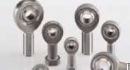
Figure 7: Ball Joint
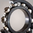
Figure 8: Ball Bearing
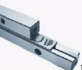
Figure 9: Roller Bearing
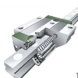
Figure 10: Roller Rail Guide
1.5 Compliant elements for constraining DoFs
1.5.1 Basic leaf springs and folded leaf springs
An example of a complaint element is shown in Figure 11.
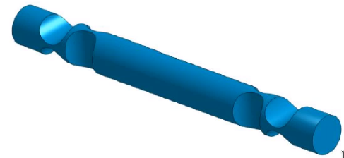
Figure 11: Example of 1dof constrained compliant element
Other types of compliant elements include:
- Leaf spring: constrains 3 dof (Figure 12)
- Folded leaf spring: constrains only 1dof (Figure 13) These are generally used in combination with other folded leaf springs.
- Flexure pivots: constrains 5 dofs (Figure 14)
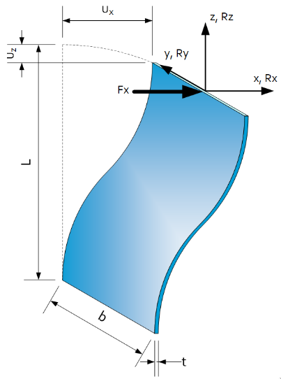
Figure 12: Leaf springs
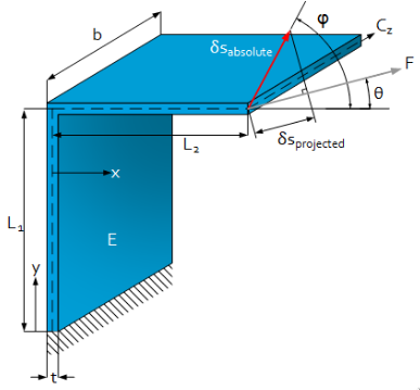
Figure 13: Folded Leaf springs
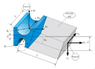
Figure 14: Flexure Pivots (5dof constrained)
1.5.2 1dof Parallel Guiding
Parallel guiding can be made using two leaf springs (Figure 15):
- 2 parallel leaf springs
- Force actuator in center of parallelism (middle of the leaf springs) to avoid coupled rotation
Sag in vertical direction as a function as the horizontal displacement. This sag is predictible and reproducible:
\begin{equation} \delta z = 0.6 \frac{x^2}{L} \end{equation}- Vertical stiffness negatively affected by displacement
- Take care of maximum buckling (Figure 16)
- Improve buckling load and Z stiffness by reinforced mid-section (Figure 17)
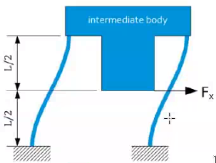
Figure 15: Parallel guiding
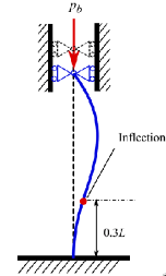
Figure 16: Example of bucklink
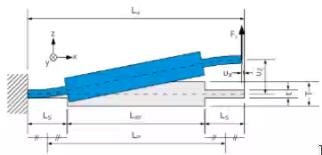
Figure 17: Reinforced leaf springs
1.5.3 Rotation Compliant Mechanism
Figure 18 shows a rotation compliant mechanism:
- 3 leaf springs
- no sensitive for thermal load on the body: as the central part heat ups and expand, the center line of the rotation stays at the same position
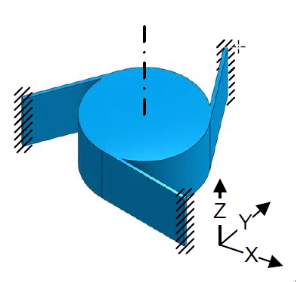
Figure 18: Example of rotation stage using leaf springs
1.5.4 Z translation
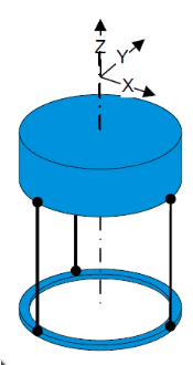
Figure 19 shows a Z translation mechanism:
- 5 struts (“needles”)
- Not sensitive for thermal loads on body
The problem is that when it moves vertical, there will also be some z rotation because the length of the strut is fixed (stiff). This parasitic rotation is however predictable.
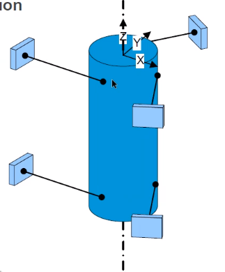
Figure 19: Z translation using 5 struts
An alternative is to use folder leaf springs (Figure 20), and this avoid the parasitic rotation.
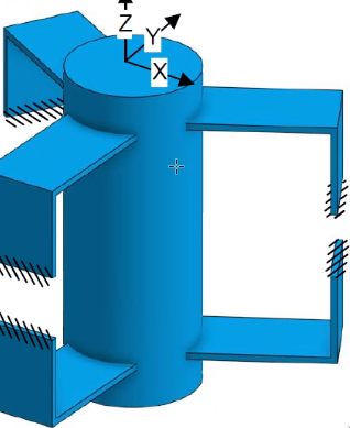
Figure 20: Z translation using 5 folded leaf springs
1.5.5 X-Y-Rz Stage
1.5.6 Compliant mechanism with only one fixed dof
The compliant mechanism shown in Figure 23 only constrain the rotation about the y-axis.
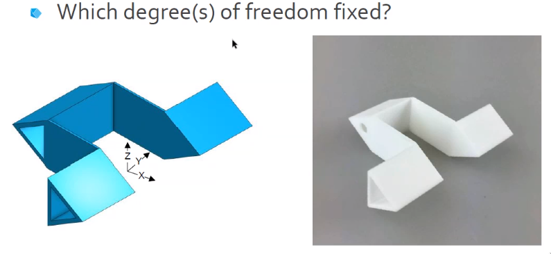
Figure 23: 5dof motion, only the Ry is constrained
1.5.7 Summary
- compliant elements enable defined movements
- Hinges or guidings can be used for small movements
- No play, No friction, No wear, No contamination
- but limited rotation, need a constant force to hold in place
1.5.8 Examples
1.5.9 Mechatronics positioning challenge
A X-Y-Rz stage is shown in Figure 26. To make this stage usable for nano-metric positioning, the following ideas where used:
- Use parallel mechanisms instead of serial one:
- no stacking of errors
- smaller, stiffer, in one plane
- Symmetry:
- Use 3 identical voice coil actuators
- Use 3 identical sensors
- Center position insensitive for temperature change
- Flexure only;
- no friction
- no play
- no wear
- no particule (important for clean rooms)
- no service
- Continuously under control:
- no alignment / crosstalk issues between axes
- voice coil / sensors combination determines performance

Figure 26: Example of X-Y-Rz positioning stage
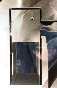
1.5.10 Case - Play Free parallel Stage
Figure 27 shows a parallel mechanism that should be converted to a compliant mechanism. Its characteristics are:
- 1mm stroke
- 1:5 lever arm
- 10kg payload
- distance between hinges: 5nmm
- thickness t: 40mm
- Material: aluminium
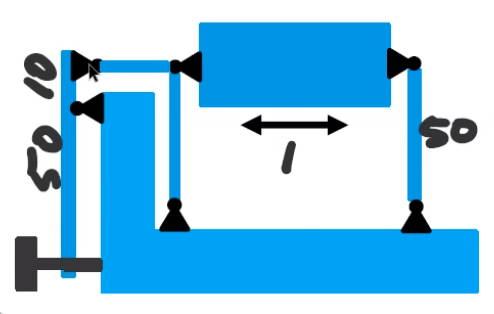
Figure 27: Example of a parallel stage that should be converting to a compliant mechanism
The goals are to:
- Make design using elastic hinges
- Maximize vertical stiffness
- Determine vertical stiffness
The solution is shown in Figure 28.
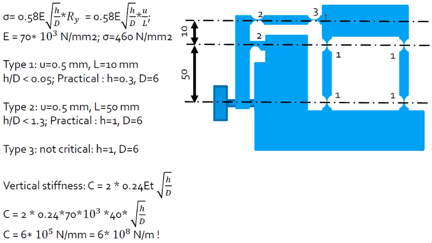
Figure 28: Case Solution
1.6 Thin plate design
1.6.1 Thin plate in torsion
Thin plates are very important for compliant mechanisms.
The torsion stiffness of a thing plate is linear with the length of the thin plate:
\begin{equation} k = \frac{G I_p}{L} \end{equation}with \(G\) the shear modulus:
\begin{equation} G \approx 0.3 E \end{equation}where \(E\) is the young modulus
Then
\begin{equation} I_p = \frac{1}{3} h t^3 = \frac{1}{3} A t^2 \end{equation}where \(A\) is the area of the cross section.
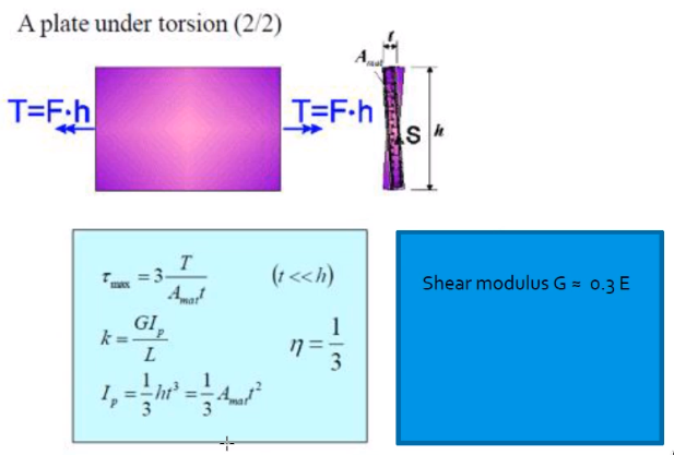
Figure 29: A plate under torsion
1.6.2 Difference between open and close profile
The close profile has much more torsional stiffness than the open profile.
Just by opening the tube, we have a much smaller torsional stiffness (but almost same axial stiffness for instance).
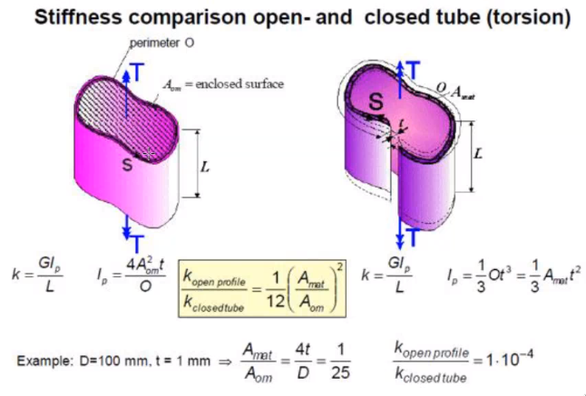
Figure 30: Stiffness comparison open and closed tube (torsion)
We have similar behavior with an open/closed box. If we remove one side of the cube shown in Figure 31, we would have much smaller torsional stiffness along the axis perpendicular to the removed side.
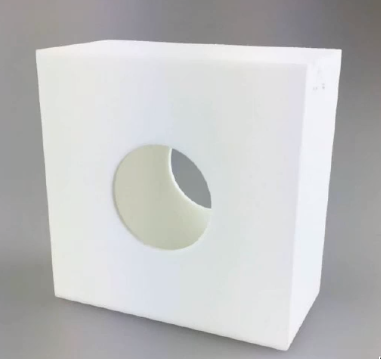
Figure 31: Closed box.
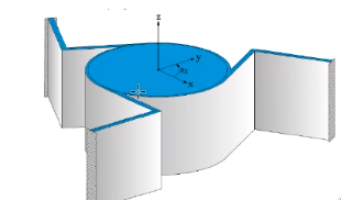
If we use triangles, we obtain high torsional stiffness as shown in Figure 32.
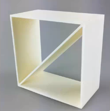
Figure 32: Open box (double triangle)
Frames are usually corresponding to open-boxes with have a small stiffness in torsion. On way to reinforce it is using triangles.
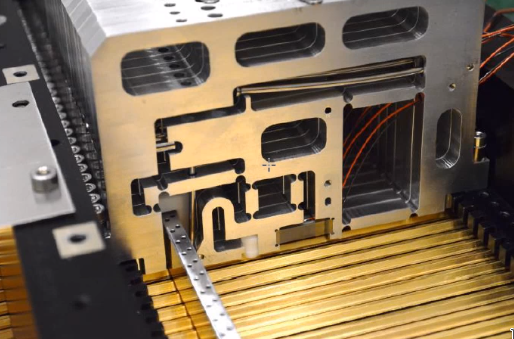
A nice way to have a 1dof flexure guiding with stiff frame is shown in Figure 33.
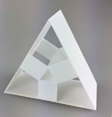
Figure 33: Box with integrated flexure guiding
2 Keynote: Mechatronic challenges in optical lithography @hans_butler
2.1 Introduction
Question: in chip manufacturing, how do developments in optical lithography impact the mechatronic design?
Main developments:
- Scanning & dual stage scanning
- Immersion
- Multiple patterning
- Extreme ultra violet lithography
2.2 Chip manufacturing loop
In this presentation, only the exposure step is discussed (lithography).
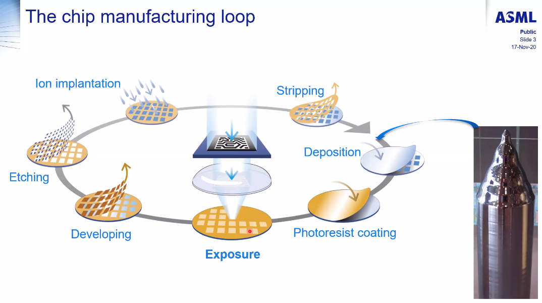
Figure 34: Chip manufacturing loop
2.3 Imaging process - Basics
- An illuminator provides light at constant wavelength \(\lambda\)
- The pattern on the reticle diffracts the light into order
- At least +/-1st orders need to be captures. This will induce a sinusoidal wave on the wafer as shown in Figure 35.
- Wafer and mast are placed on high accuracy moving stages
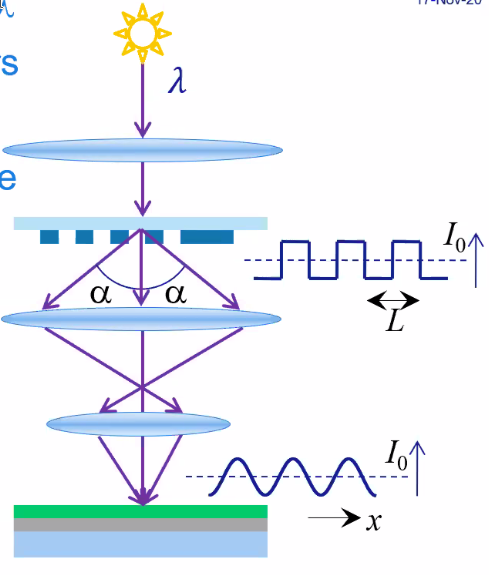
Figure 35: Imaging process - basics
2.4 From stepper to scanner
Before, one chip was illumating at a time, but people wanted to make bigger chips. However, if was difficult to make larger lenses.
The solution was to use a scanner, were both the mask and wafer are on moving stages. This implied many requirements in dynamics and accuracy!
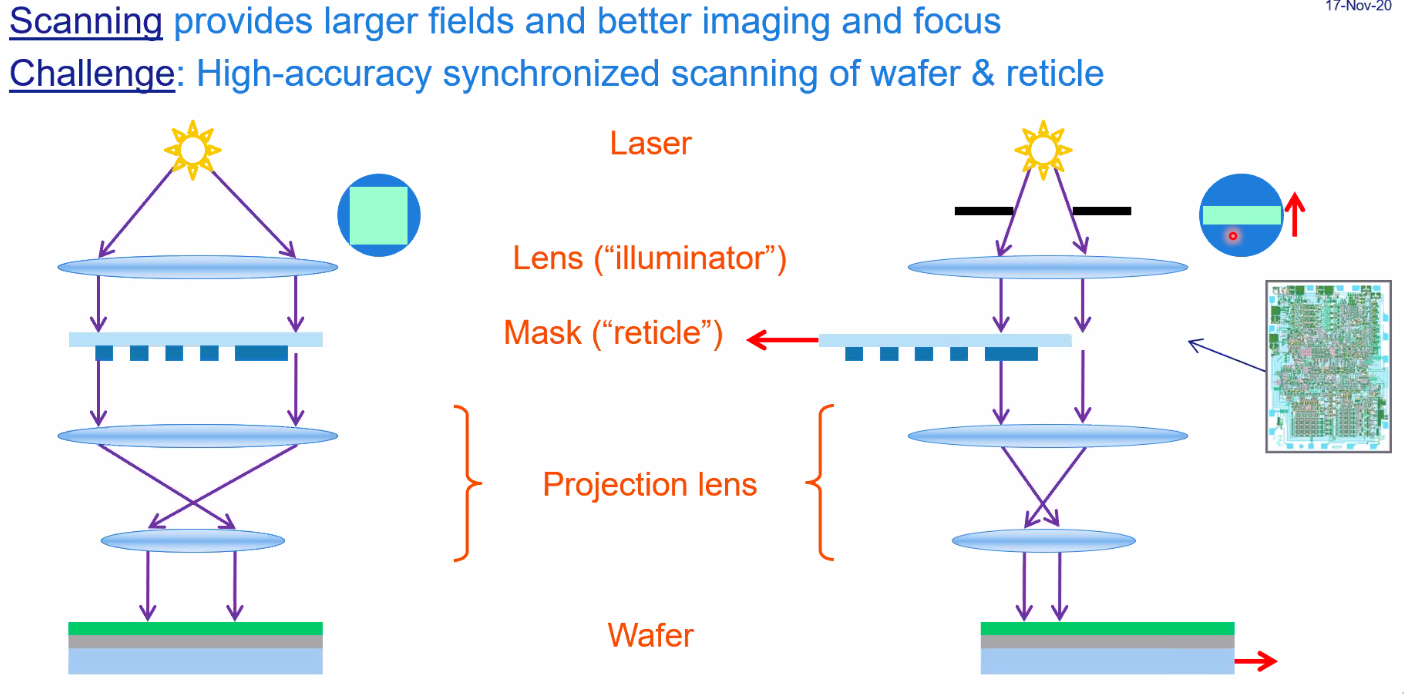
Figure 36: From stepper to scanner
2.5 Dual stage scanners
Both the reticle stage and wafer stage are moving. In order to have the same throughput, higher stage accelerations are required.
This implies some mechatronics challenges:
- higher stage acceleration
- higher accuracy
- interaction between stages
Which are solved by:
- Larger forces => balance masses
- Stage dynamical design for high bandwidth control
- Control coupling between stages (one control system can act as a disturbance to another controlled system => feedforward)
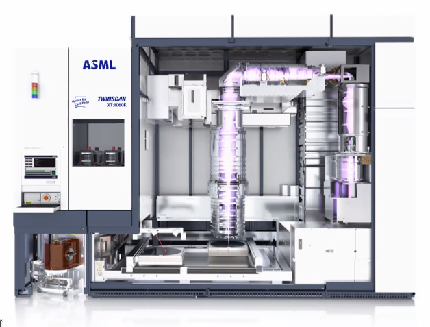
Figure 37: Machine based on the dual stage scanners
2.6 Immersion technology
Water is used between the lens and the wafer to increase the “NA” and thus decreasing the “critical dimension”.
The “hood” is there to prevent any bubble to enter the illumination area (Figure 38). The position of the “hood” is actively control to follow the wafer stage (that can move in z direction and tilt).
Three solutions are used for the positioning control of the “hood” system (Figure 39):
- Disturbance decoupling
- Iterative learning control
- Feed-forward control from the Wafer control signal
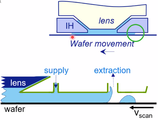
Figure 38: Hood System
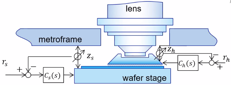
Figure 39: Control system for the “hood”
2.7 Multiple Patterning
The multiple patterning approach adds few mechatronics challenges:
- Position accuracy limited to ~4nm due to interferoemter position measurement (variation of temperature/pressure of air)
- Stage swap is complex and time-consuming
This was solved by:
- Using encoder instead of interferometers
- Use long stroke motor: h-stage => new wafer stage concept
2.8 Machine layout
Each stage is controlled with 6dof lorentz short stroke actuators (Figure 40). The magnet stage can move horizontally (due to reaction forces of the wafer stages): it asks as a balance mass.
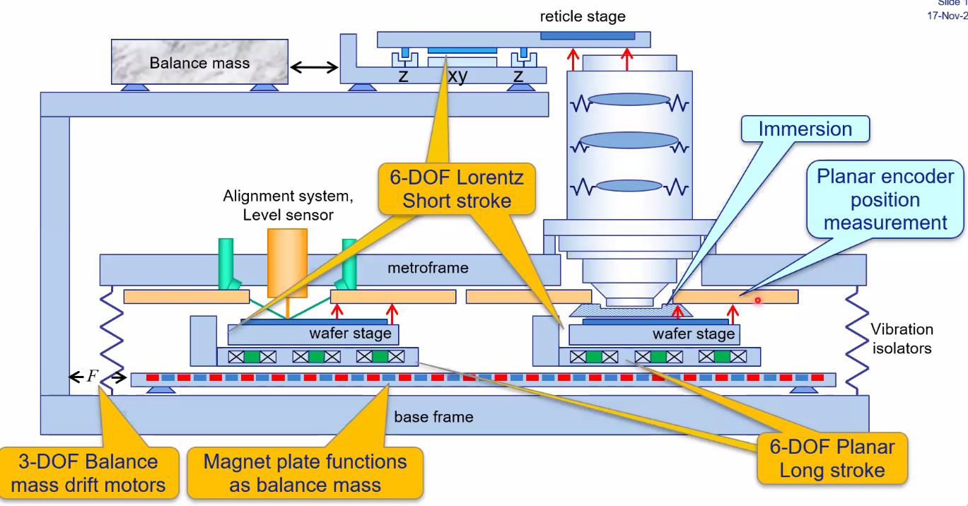
Figure 40: Machine layout
2.9 EUV Lithography
Vacuum is required which implies:
- no bearings
- no cooling
All the optics are reflective:
- extremely accurately polished
- challenge: keep mirrors optimally positioned
Wafer stage:
- Move at high speed and accelerations
- Challenge: in vaccum
- Solved by: machanically suspended balance mass, and interferoemter position meaured can be used because it is in vacuum now
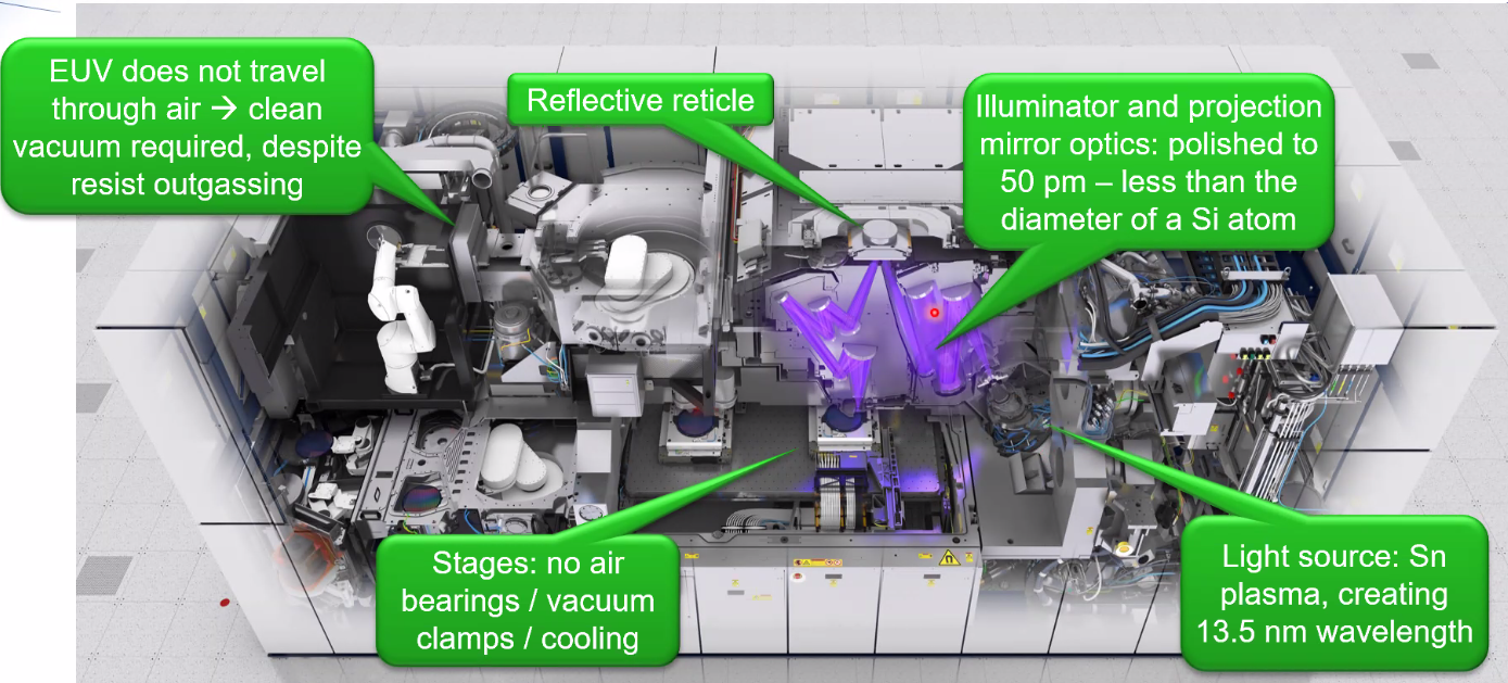
Figure 41: Schematic of the ASML EUV machine
2.10 The future: high-NA EUV
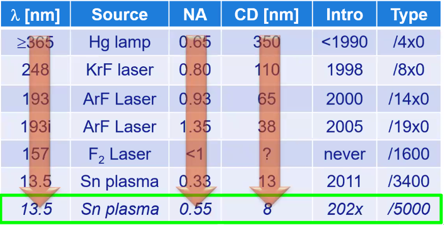
Figure 42: The CD will be 8nm
In order to do so, high “opening” of the optics is required which is very challenges because the reflectiveness of mirror is decreasing as high angle of incidence (Figure 43).
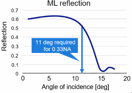
Figure 43: Change of reflection of a mirror as a function of the angle of indicence
2.11 Challenges for future Optical Lithography machines
Challenges:
- Double wafer stage acceleration
- Much bigger mirrors
- Tighter accuracy specifications despite
Solutions:
- Stage and mirror dynamics, high bandwidth control
- Dynamics architecture: improved isolation, multiple isolate sets
- Heating compensation
2.12 Conclusion
The conclusions are:
- Lithographic tools are the main enabler for over shrinking device sizes
- New (optical) requirements lead to new mechatronic challenges:
- Larger fields / better imaging: from stepping to scanning
- Larger wafer size: dual stage scanners
- Immersion: wafer stage & hood control
- Multiple patterning: planar motors and encoder technology
- EUV: all-vacuum stages
- High-NA EUV: new optics, much larger accelerations
3 Keynote: High precision mechatronic approaches for advanced nanopositioning and nanomeasuring technologies @eberhard_manske
3.1 Coordinate Measurement Machines (CMM)
Examples of Nano Coordinate Measuring Machines are shown in Figure 44.
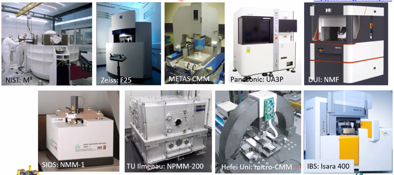
Figure 44: Example of Coordinate Measuring Machines
3.2 Difference between CMM and nano-CMM
With classical CMM, the Abbe-principle is not fulfilled in the x and y directions (Figure 45).
The Abbe error can be determined with:
\begin{equation} \Delta l_{x,y,z} = l_{x,y,z} \sin \Delta \phi_{x,y,z} \end{equation}Even with the best spindle: \(l_{x,y} = 100 mm\) and \(\Delta \phi = 2 \text{arcsec}\), we obtain an error of:
\begin{equation} \Delta l = 0.1 \mu m \end{equation}which is not compatible with nano-meter precisions.
Then, the classical CMM will not work for nano precision
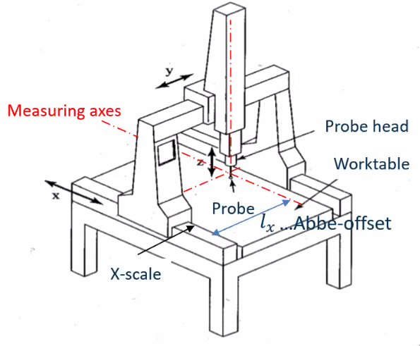
Figure 45: Schematic of a CMM
3.3 How to do nano-CMM
High precision mechatronic approaches are required for advanced nano-positionign and nano-measuring technologies:
- High precision measurement concept
- High precision measurement systems
- High precision nano-sensors
Combined with:
- Advanced automatic control
- Advanced measuring strategies
3.4 Concept - Minimization of the Abbe Error
In order to minimize the Abbe error, the measuring “lines” should have a common point of intersection (Figure 46).
The 3D-realization of Abbe-principle is as follows:
- 3 interferometers: cartesian coordinate system
- probe located as the intersection point of the interferometers
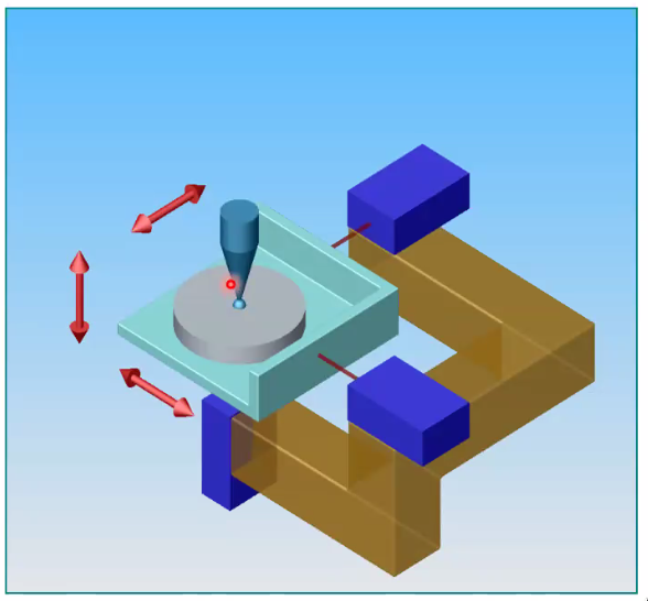
Figure 46: Error minimal measuring principle
3.5 Minimization of residual Abbe error
Still some residual Abbe error can happen as shown in Figure 47 due to both a change of angle and change of position.
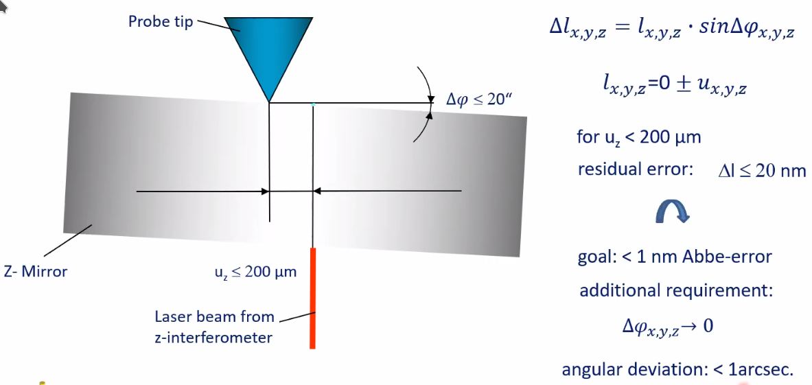
Figure 47: Residual Abbe error
3.6 Compare of long travel guiding systems
In order to have the Abbe error compatible with nano-meter precision, the precision of the spindle should be less and one arcsec which is not easily feasible with air bearing of precision roller bearing technologies as shown in Figure 48.
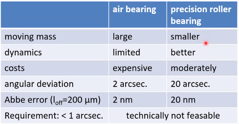
Figure 48: Characteristics of guidings
3.7 Extended 6 DoF Abbe comparator principle
The solution used was to measure in real time the angles of the frame using autocollimators as shown in Figure 49 and then to minimize this tilt by close loop operation with additional actuators.
The angular measurement error and control is less than \(0.05 \text{arcses}\) which make the residual Abbe error:
\begin{equation} \Delta l < 0.05\,nm \end{equation}Without an error-minimal approach, nano-meter precision cannot be achieved in large areas.

Figure 49: Use of additional autocollimator and actuators for Abbe minimization
3.8 Practical Realisation
A practical realization of the Extended 6 DoF Abbe comparator principle is shown in Figure 50.
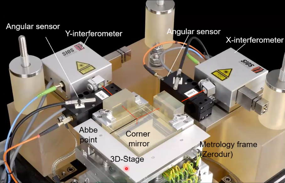
Figure 50: Practical Realization of the
3.9 Tilt Compensation
To measure compensate for any tilt, two solutions are proposed:
- Use a zero point angular auto-collimator (Figure 51)
- Resolution: 0.005 arcsec
- Stability (1h): < 0.05 arcsec
- 6 DoF laser interferoemter (Figure 52)
- Resolution: 0.00002 arcsec
- Stability (1h): < 0.00005 arcsec
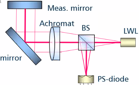
Figure 51: Auto-Collimator
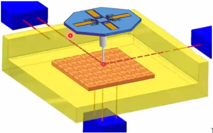
Figure 52: 6 Interferometers to measure tilts
3.10 Comparison of long travail guiding systems - Bis
Now, if we actively compensate the tilts are shown previously, we can fulfill the requirements as shown in Figure 53.
Measurement and control technology to minimize Abbe errors to achieve:
- sub-nanometer precision
- smaller moving mass
- better dynamics
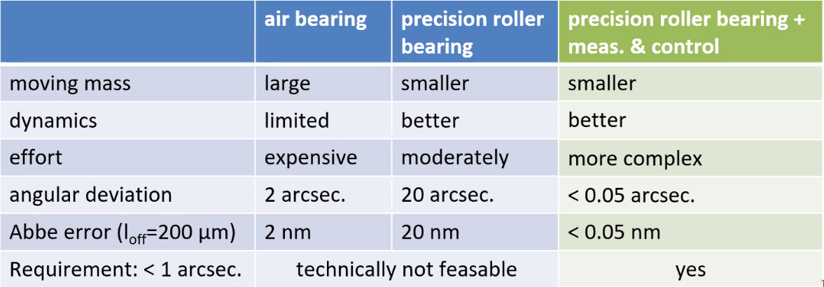
Figure 53: Characteristics of the tilt compensation system
3.11 Drive concept
Usually, in order to achieve a large range over small resolution, each axis of motion is a combination of a coarse motion and a fine motion stage. The coarse motion stage generally consist of a stepper motor while the fine motion is a piezoelectric actuator.
The approach here is to use an homogenous drive concept for increase dynamics (Figure 54).
Only one linear voice coil actuator is used which with large moving range and sub-nanometer resolution can be achieve at one time.
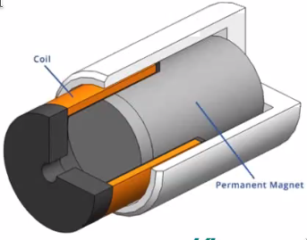
Figure 54: Voice Coil Actuator
3.12 NPMM-200 with extended measuring volume
The NPMM-200 machine can be seen in Figure 55.
Characteristics:
- Measuring range: 200 mm x 200 mm x 25 mm
- Resolution: 20 pm
- Abbe comparator principle
- 6 laser interferometers
- Active angular compensation
- Position uncertainty < 4 nm
- Measuring uncertainty up to 30 nm
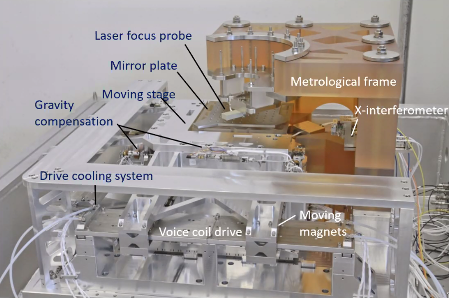
Figure 55: Picture of the NPMM-200
The NPMM-200 actually operates inside a Vacuum chamber as shown in Figure 56.
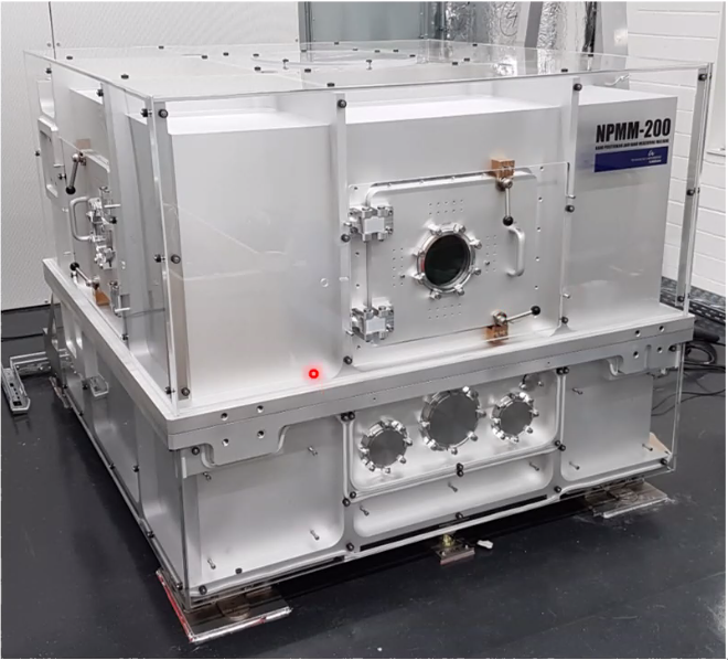
Figure 56: Vacuum chamber used
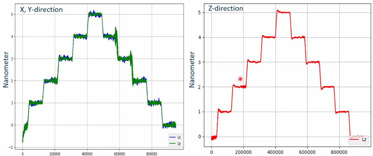
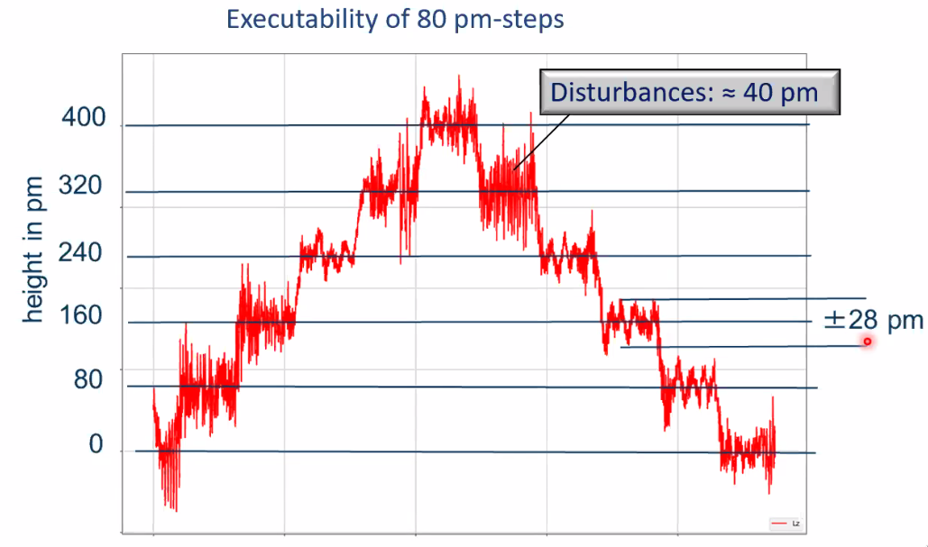
3.13 measurement capability
3.14 Extension of the measuring range (700mm)
If the measuring range is to be increase, there are some limits of the moving stage principle:
- large moving masses (~300kg)
- powerful drive systems required
- nano-meter position capability problematic
- large heat dissipation in the system
- dynamics and dynamic deformation
The proposed solution is to use inverse dynamic concept for minimization of moving masses.
3.15 Inverse kinematic concept - Tetrahedrical concept
The proposed concept is shown in Figure 59:
- mirrors and object to be measured are fixed
- probe and interferometer heads are moved
- laser beams virtually intersect in the probe tip
- Tetrahedrical measuring volume
This fulfills the Abbe principe but:
- large construction space
- difficult guide and drive concept
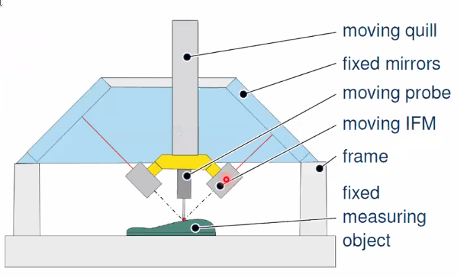
Figure 59: Tetrahedrical concept
3.16 Inverse kinematic concept - Scanning probe principle
An other concept, the scanning probe principle is shown in Figure 60:
- cuboidal measuring volume
- Fixed x-y-z mirrors
- moving measuring head
- guide and drive system outside measuring volume
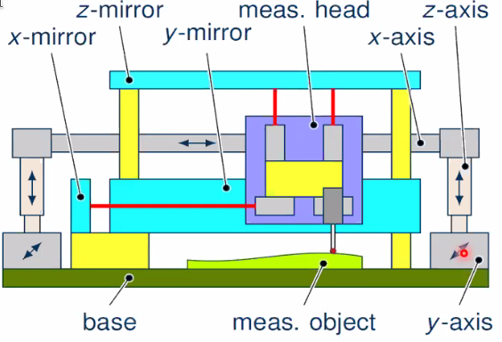
Figure 60: Scanning probe principle
3.17 Inverse kinematic concept - Compact measuring head
In order to minimize the moving mass, compact measuring heads have been developed. The goal was to make a lightweight measuring head (<1kg)
The interferometer used are fiber coupled laser interferometers with a mass of 37g (Figure 61).
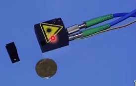
Figure 61: Micro Interferometers
The concept is shown in Figure 62:
- 6dof interferometers are used
- one micro-probe
- the total mass of the head is less than 1kg
There is some abbe offset between measurement axis of probe and of interferometer but Abbe error compensation by closed loop control of angular deviations is used.
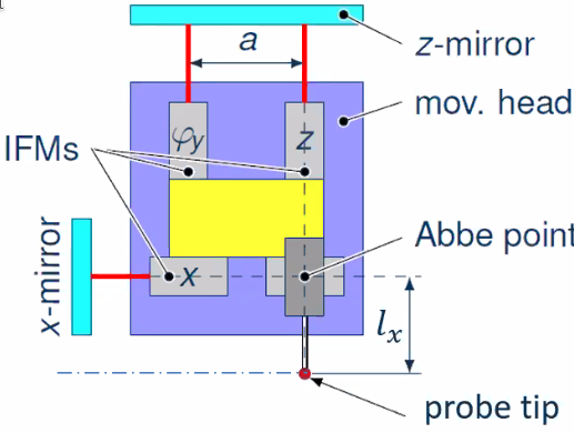
3.18 Inverse kinematic concept - Scanning probe principle
As shown in Figure 63, the abbe error can be compensated from the two top interferometers as: \[ \text{for } l_x = a: \quad \Delta l_{\text{Abbe}} = \Delta l_{\text{int}} \] Thus the tilt and Abbe errors can be compensated for with sub-nm resolution.
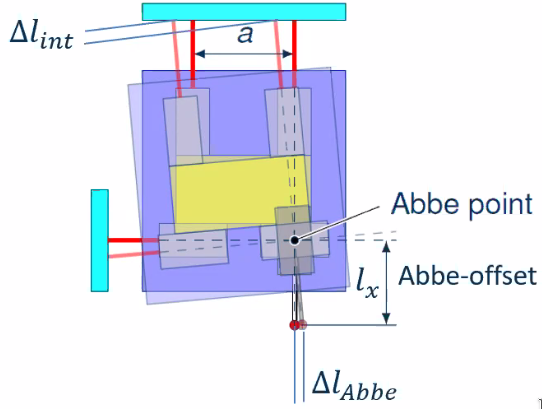
Figure 63: Use of the interferometers to compensate for the Abbe errors
3.19 Conclusion
Proposed approaches to push the nano-positioning and nano-measuring technology:
- Measurement and control technology to minimize Abbe errors
- Homogeneous drive concept for increased dynamics
- Inverse kinematic concept for minimization of moving mass
- Abbe-error compensation by closed loop control of angular deviations
4 Designing anti-aliasing-filters for control loops of mechatronic systems regarding the rejection of aliased resonances @ulrich_schonhoff
4.1 The phenomenon of aliasing of resonances
Weakly damped flexible modes of the mechanism can limit the performance of motion control systems.
For discrete time controlled systems, there can be an additional limitation: aliased resonances which are rarely discussed.
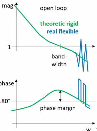
Figure 64: Example of high frequency lighlty damped resonances
The aliasing of signals is well known (Figure 65).
However, aliasing in systems can also happens and is schematically shown in Figure 66.
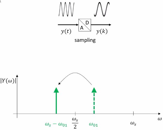
Figure 65: Aliasing of Signals
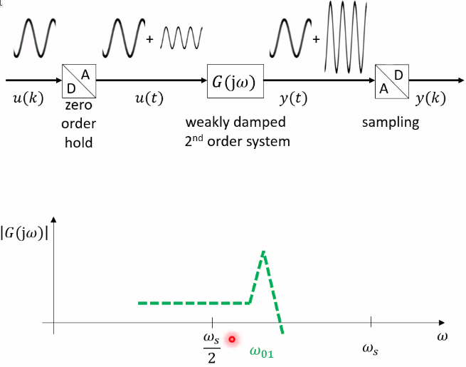
Figure 66: Aliasing of Systems
The poles of the system will be aliased and their location will change in the complex plane as shown in Figure 67.
More precisely:
- the imaginary parts of the poles mirror about the Nyquist frequency
- the real parts of the poles remain equal
Therefore, the damping of the aliased resonances are foreseen to have larger dampings.
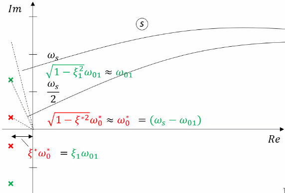
Figure 67: Aliasing of poles in the complex plane
Let’s consider two systems with a resonance:
- below the Nyquist frequency (blue dashed)
- above the Nyquist frequency (green dashed)
Then looking at the same systems in the digital domain, one can see thathen the resonance is above the Nyquist frequency (Figure 68):
- the resonance mirrors
- the damping is increased
Therefore, when identifying a low damped resonance, it could be that it comes form a high frequency low damped resonance.
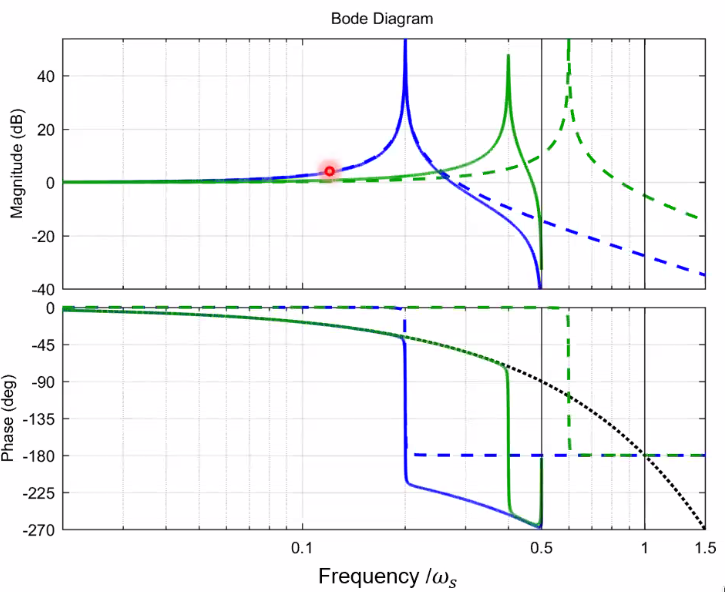
Figure 68: Aliazed resonance shown on the Bode Diagram
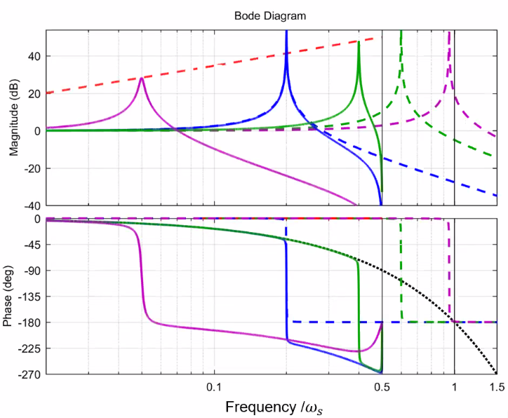
Figure 69: Higher resonance frequency
4.2 Nature, Modelling and Mitigation of potentially aliasing resonances
The aliased modes can for instance comes from local modes in the actuators that are lightly damped and at high frequency (Figure 70)
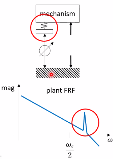
Figure 70: Local vibration mode that will be alized
The proposed idea to better model aliasing resonances is to include more modes in the FEM software as shown in Figure 71 and then perform an order reduction in matlab.
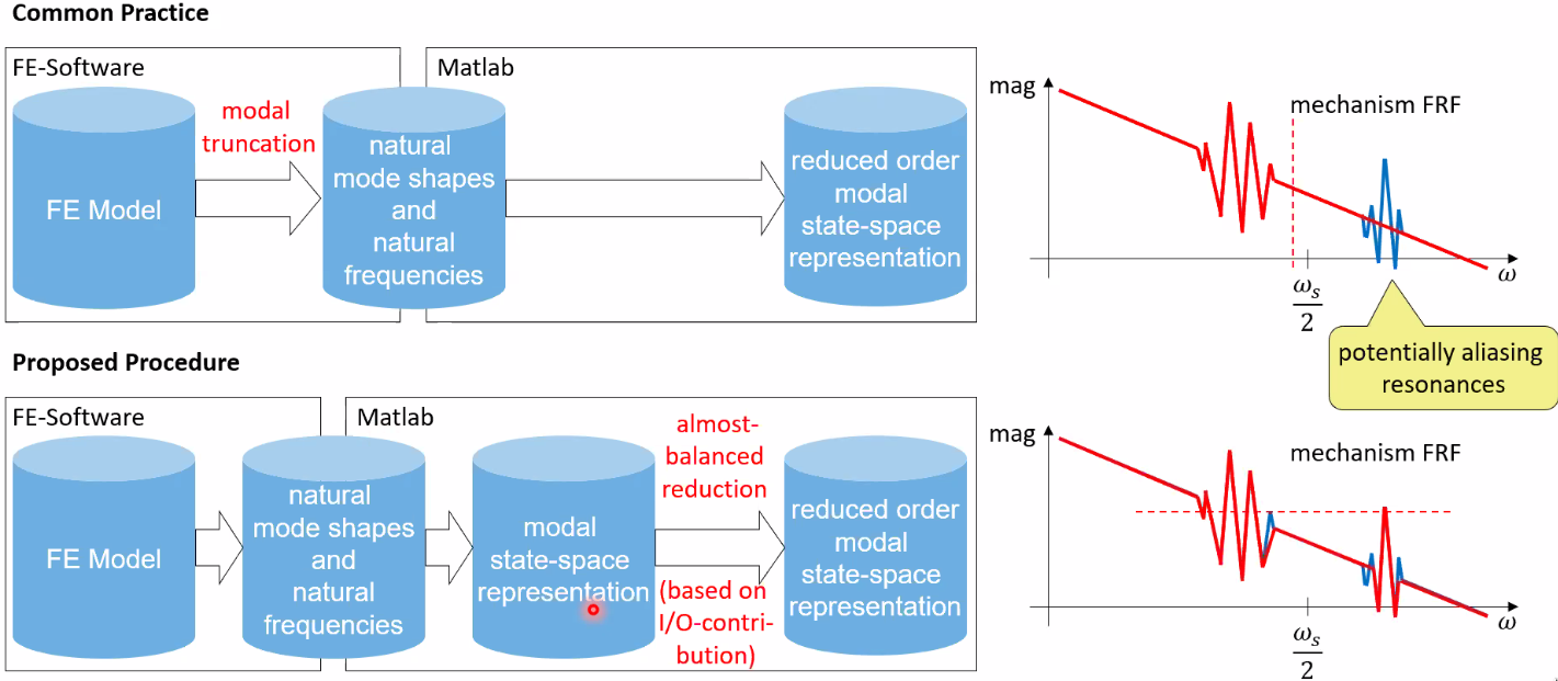
Figure 71: Common procedure and proposed procedure to include aliazed resonances
4.3 Anti aliasing filter design
4.3.1 Introduction
- Anti-aliasing filtering can be used to reject aliasing of resonances and to maintain the stability of the control loop
- However, its phase lag deteriorates the control loop performances:
- Thus, the anti-aliasing filter should be targeted at sufficient rejection at least possible phase lag
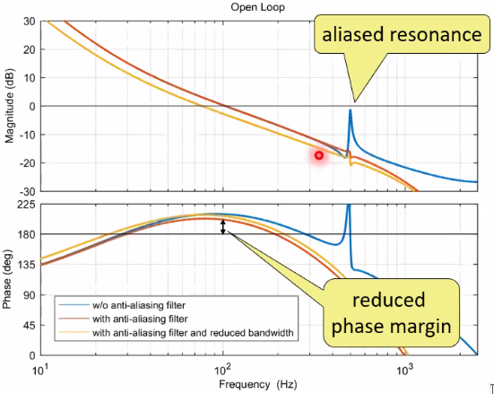
Figure 72: Example of the effect of aliased resonance on the open-loop
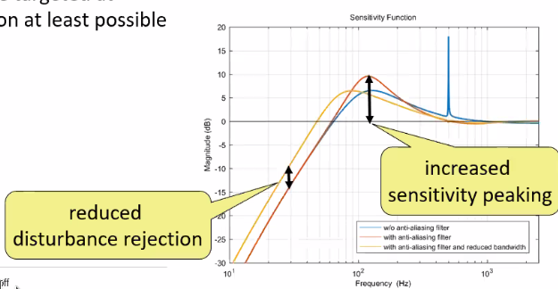
Figure 73: Example of the effect of aliased resonance on sensitivity function
4.3.2 Concept of equivalent delay
Concept:
At frequencies well below its poles and zeros, a continuous time filter \(F(j\omega)\) shows almost linear phase:
\begin{equation} \arg\big( F(j\omega) \big) \approx -T_e \omega \end{equation}Thus, the phase lag of the filter can be fairly correctly represented by a time delay (below the pole frequency). The equivalent delay is:
\begin{equation} T_e = \sum_{i=1}^{N_p} \frac{\xi_{pi}}{\omega_{0pi}} - \sum_{i=1}^{N_z} \frac{\xi_{zi}}{\omega_{0zi}} \end{equation}- where \(\omega_{0pi}\) is the natural frequency \(\xi_{pi}\) is the damping of the \(N_p\) poles of \(F(s)\). Similarly, \(\omega_{0zi}\) is the natural frequency \(\xi_{zi}\) is the damping of the \(N_z\) zeros of \(F(s)\).
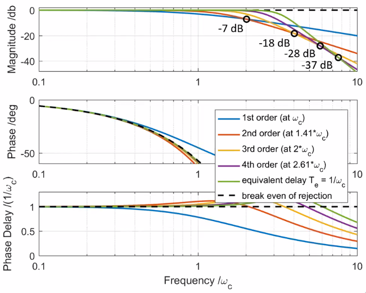
Examples (Figure 74):
- First order low pass filter: \[ \xi_p = 1 \Rightarrow T_e = \frac{1}{\omega_c} \]
- Second order Butterworth low pass filter: \[ \xi_p = \frac{1}{\sqrt{2}} \Rightarrow T_e = \sqrt{2} \frac{1}{\omega_c} \]
- First order lead: \[ \xi_z = 1 \Rightarrow T_e = - \frac{1}{\omega_c} \]
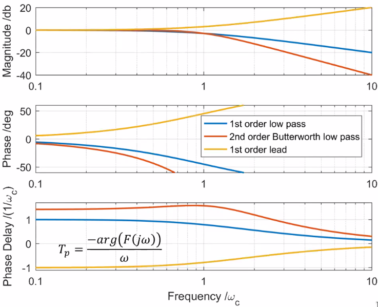
Figure 74: Magnitude, Phase and Phase delay of 3 filters
4.3.3 Budgeting of phase lag
The budgeting of the phase lag is done by expressing the phase lag of each element by a time delay (Figure 75)
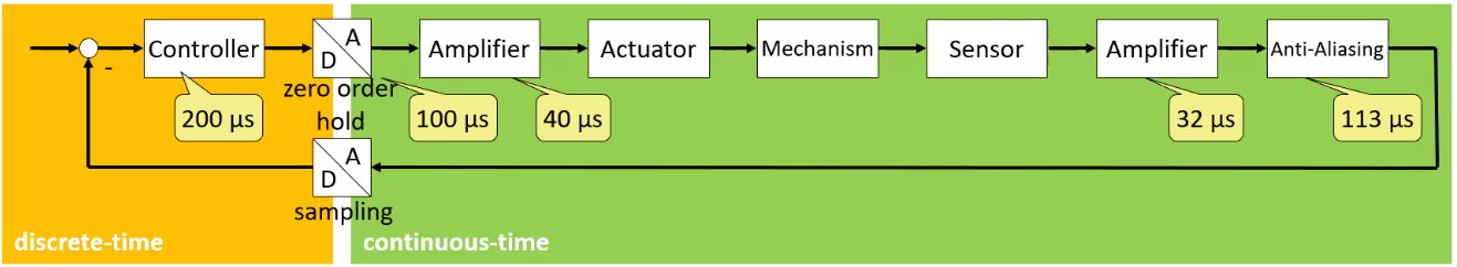
Figure 75: Typical control loop with several phase lag / time delays
The equivalent delay of each element are listed in Figure 76.
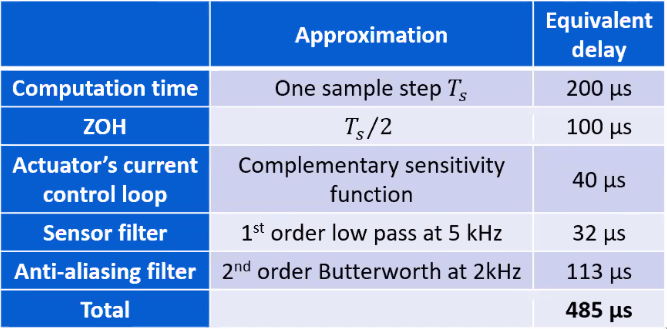
Figure 76: Equivalent delay for all the elements of the control loop
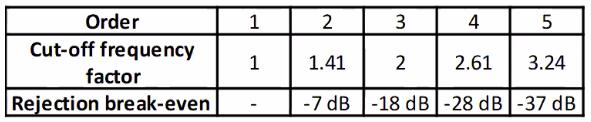
4.3.4 Selecting the filter order
4.3.5 Reducing the phase lag
The equivalent delay of a low pass (here second order) depends on its damping, since: \[ T_e = -2 \frac{\xi_{zi}}{\omega_{0zi}} \]
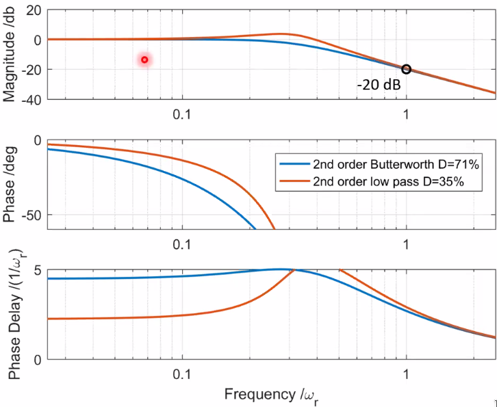
Figure 79: Change of the phase delay with the damping of the filter
4.4 Conclusion
The phenomenon of aliasing of resonances:
- Aliasing of resonances is an issue in discrete-time controlled mechatronic systems and can limit the performance and even render the closed loop system unstable
- Resonances above the Nyquist Frequency appear aliased at mirrored frequency for the discrete-time controller
- Aliased resonances show increased damping compared to the original resonances
- To find out if a resonance is an aliased one or not, change the sampling frequency and see if the frequency of the resonance is changing or not
Nature, modelling and mitigation of potentially aliasing resonances:
- The origin are typically local resonances of the sensor and actuator components
- Careful modelling and selecting dominant modes above the Nyquist frequency is commended
Anti-aliasing filter design:
- Anti-Aliasing filter design is the trade-off between rejection and phase-lag
- The concept of equivalent delay allows to budget and design the phase lag
- The order selection of anti alising-filter based on the required rejection is shown
- Several approaches to reduce overall phase lag are presented
5 Flexure positioning stage based on delta technology for high precision and dynamic industrial machining applications @mikael_bianchi
5.1 Introduction
- Goal: flexure positioning stage to do high precision and high dynamic/acceleration positioning. The control architecture should be as simple as possible.
- Application: micromachinign for fabrication of 3d structures
- Possible field: watch industry, electronics, optics, …
- Possible technologies: laser, milling, electro discharge machine
- Objectives: improve the productivity reaching high accelerations at high precision
5.2 Design
5.2.1 Description of the Delta robot
Technical choice: flexure based delta robot (Figure 80).
- Advantages: high mechanical precision without backlash
- Disadvantage: the motion is coupled, some transformations are required from motor coordinates to machine coordinates (Figure 81)
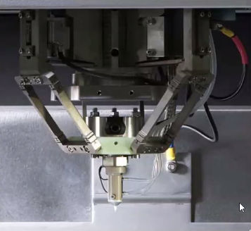
Figure 80: Picture of the Delta Robot
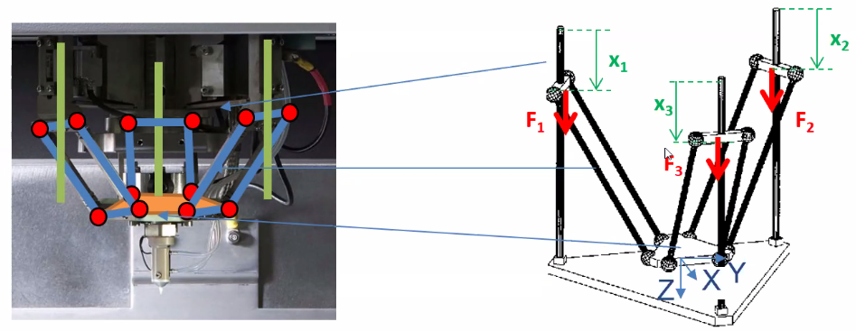
Figure 81: x1, x2 x3 are the motor positions. f1,f2 f3 are the force motors. x,y,z are the position of the final point in cartesian coordinates
5.2.2 Modelling and validation of the delta robot
Lagrange equations are used to model the dynamics of the delta robot. The motor positions are used as the general coordinate system.
The system is then linearized around the working point (Figure 82).
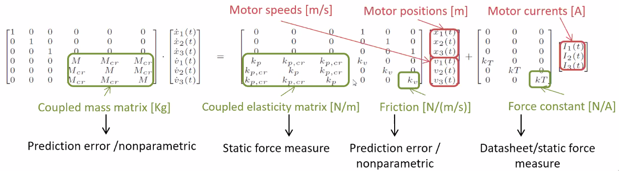
Figure 82: Linearized equations of the Delta Robot
Then the parameters are identified from experiment (Figure 83).
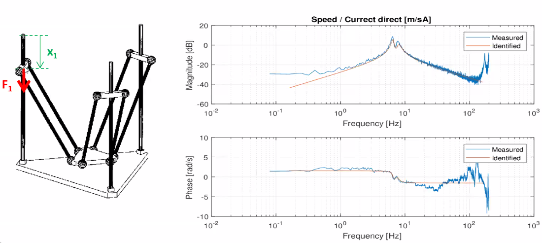
Figure 83: Identification fo the transfer function from \(F_1\) to \(x_1\)
The measurement of the coupling is move complicated as shown in Figure 84.
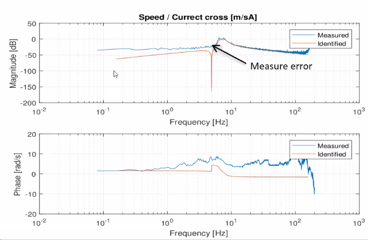
Figure 84: Problem of identifying the coupling between F1 and x2 at low frequency
5.2.3 Control design for high trajectory tracking
Control requirements:
- Precise position control of the coupled system (+/-10nm steps)
- Minimal trajectory error at high frequency (+/- 100nm at +/- 1g acceleration)
- Higher resonances attenuation
- Whole motion system is considered as a standard cartesian XYZ axes for the user (do the inverse/forward kinematics inside the control architecture)
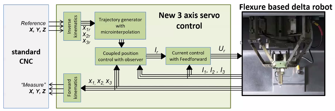
Figure 85: Control concept used for the Delta robot
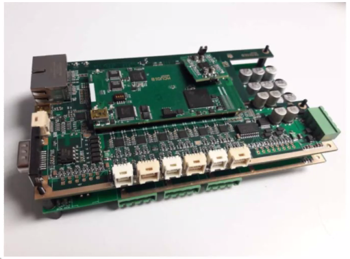
5.2.4 Electronic board
A 3 axis servo control board as been developed (Figure 86) which includes:
- identification algorithm of the coupled system integrated in the board
- interpolator for sensors
 ]
]
5.3 Results
5.3.1 Current control
Step response of the current control loop is shown in Figure 86.
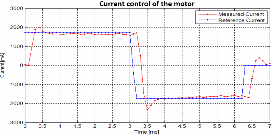
Figure 86: Step response for the current control loop
5.3.2 Trajectory tracking: results with laser interferometer and encoder
XY renishaw interferometers used to verify the performance of the system (Figure 87).
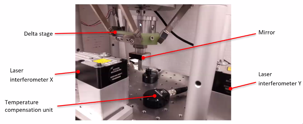
Figure 87: Experimental setup to verify the performances of the system
Some results are shown in Figures 88, 89 and 90.
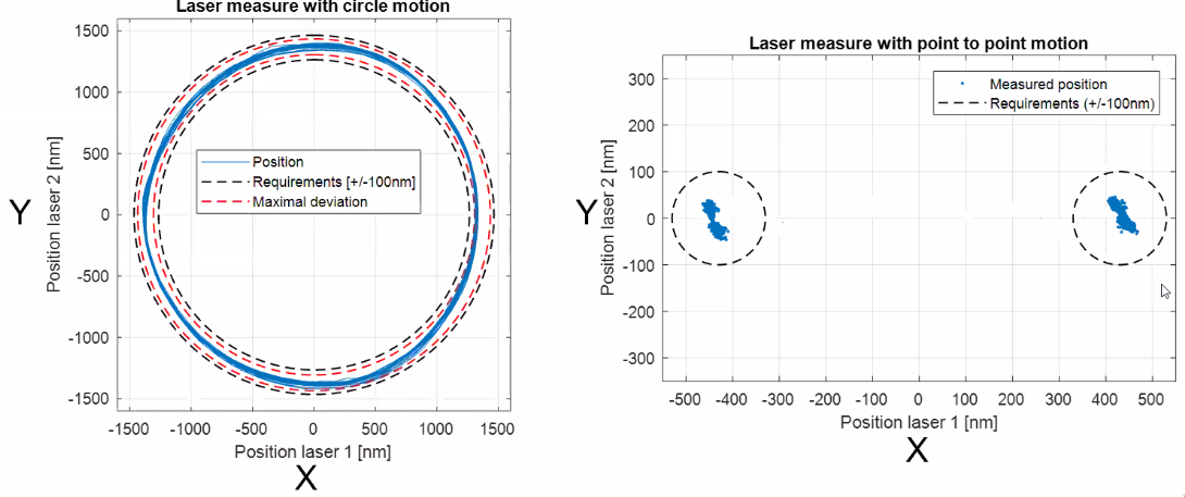
Figure 88: Circuit motion results and point to point motion results
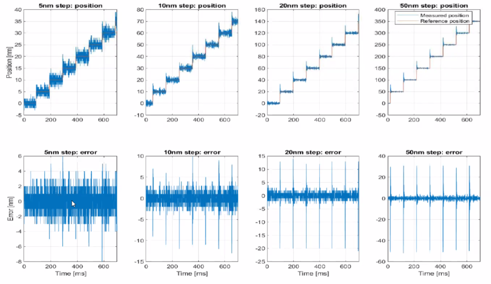
Figure 89: Step response of the system
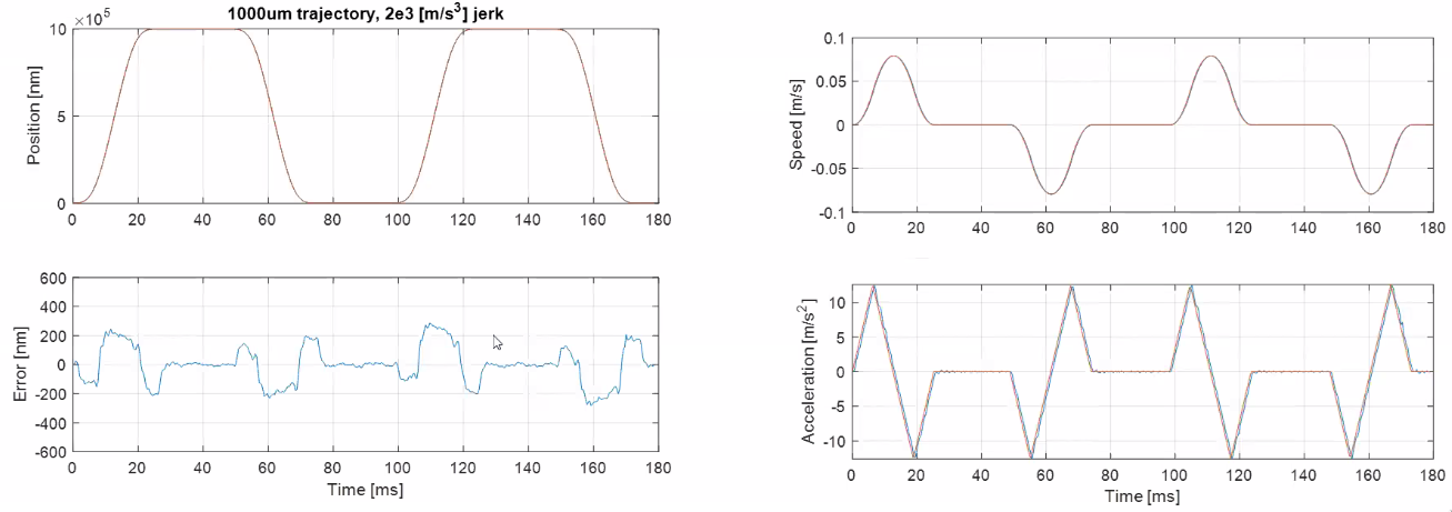
Figure 90: Measured dynamical errors
5.4 Conclusion
As a conclusion, here are the identified conditions for precise and high dynamic positioning:
- Mechanics without backlash and resonances in higher frequency
- Feedforward with correct parameters
- High bandwidth position control and precise encoder
- Low noise current sensors and high bandwidth current control
Resonances at mid frequencies are an issue for further improvements.
6 Multivariable performance analysis of position-controlled payloads with flexible eigenmodes @luca_mettenleiter
6.1 Motivation
Flexible eigenmodes are present in every system component and leads to::
- controller bandwidth limitation (Figure 91)
- additional cross-coupling in the system behavior (Figure 92)
=> can lead to stability problems
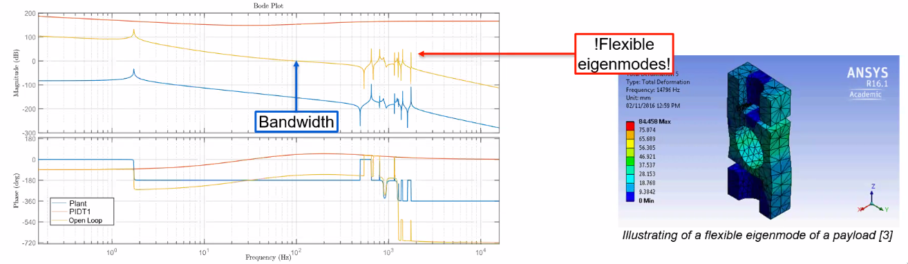
Figure 91: Limitation of the control bandwidth due to flexible eigenmodes
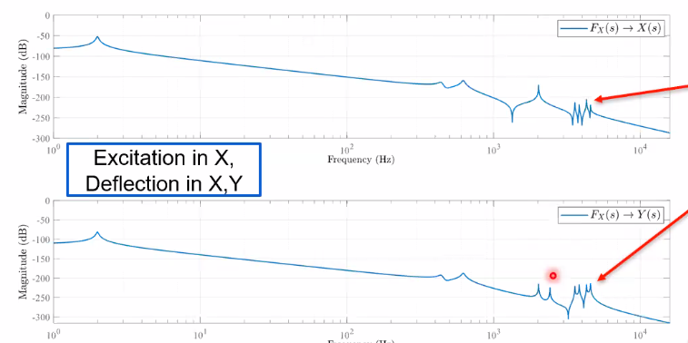
Figure 92: Coupling due to flexible eigenmodes
In order to estimate the performances of a system, the sensitivity function can be used (Figure 93).
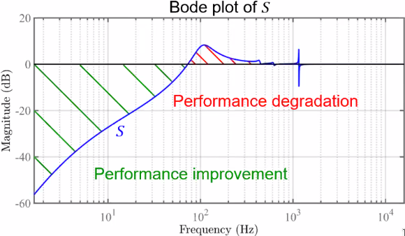
Figure 93: Bode plot of a typical Sensitivity function
6.2 Performance analysis with different sensitivity functions
There are different way to analyse the sensitivity function base on different plants (Figure 94):
- the full system (complicated): \[ L_{full} = \begin{bmatrix}L_{11} & L_{12} \\ L_{21} & L_{22} \end{bmatrix} \]
- the diagonal system (ignoring interaction) \[ L_{diag} = \begin{bmatrix}L_{11} & 0 \\ 0 & L_{22} \end{bmatrix} \]
- the loop interaction system (the one proposed here) \[ L^{LI} = \begin{bmatrix}L_1^{LI} & 0 \\ 0 & L_2^{LI} \end{bmatrix} \]
The loop interaction methods created a SISO system that also represents the coupling in the system. One loop is closed at a time, and the coupling effects are taken into account.
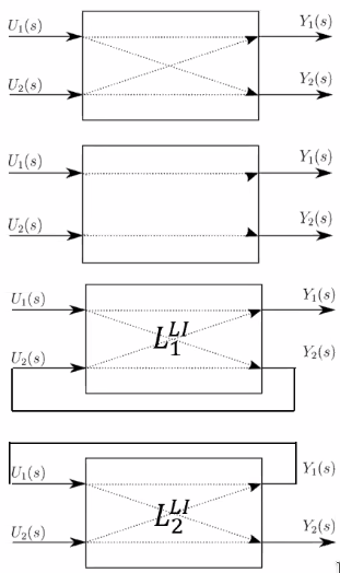
Figure 94: Visual representation of the three systems
6.3 Example system
In order to compare the use of the three systems to estimate the performances of a MIMO system, the system shown in Figure 95 is used. The 4 top masses are used to represent a payload that will add coupling in the system due to its resonances.
A diagonal PID controller is used.
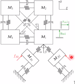
Figure 95: Schematic representation of the example system
The bode plot of the MIMO system is shown in Figure 96 where we can see the resonances in the off-diagonal elements.
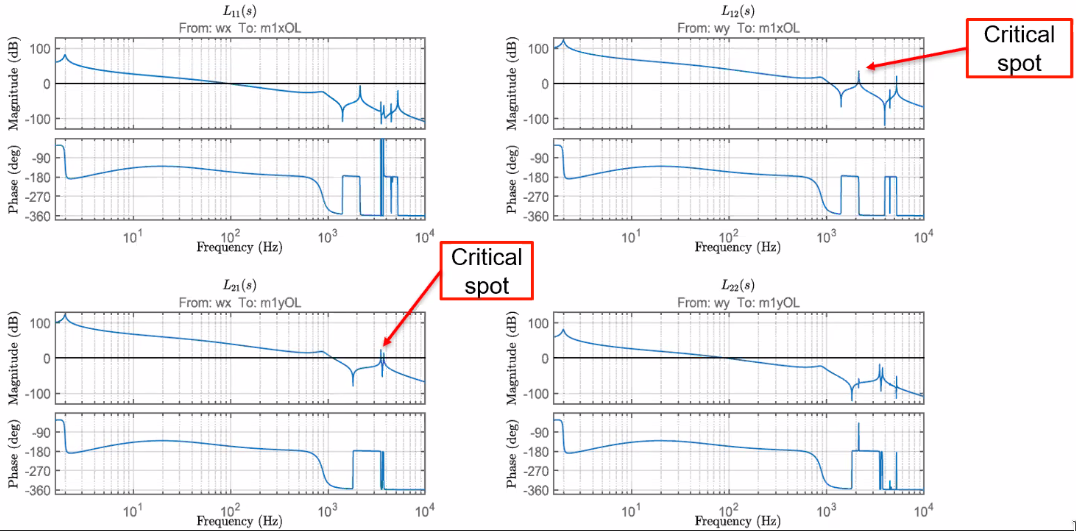
Figure 96: Bode plot of the full MIMO system
In Figure 97 is shown that the sensitivity function computed from the SISO system is not correct. Whereas for the “interaction method” system, it is correct and almost match the full system sensibility. However, as expected, the off-diagonal sensibilities are not modelled.
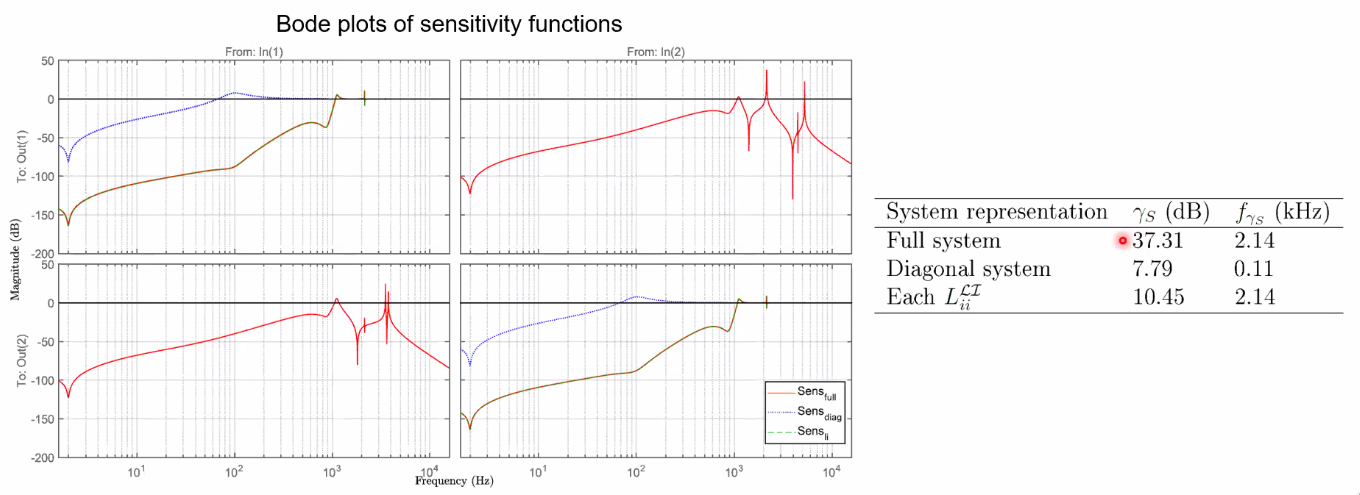
Figure 97: Bode plots of sensitivity functions
6.4 Conclusion
The conclusion are the following and summarized in Figure 98:
- Choice of suitable analysis method is key concept in mechatronics engineering
- Various methods for analysis of multivariable systems available:
- Full system always delivers reliable information, but much analysis effort
- Loop interaction method delivers reliable information, only if the system is weakly or symmetrically coupled
- Diagonal system delivers unreliable information, as it does not take multivariable character into account
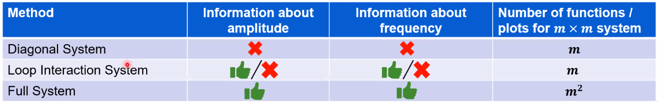
Figure 98: Comparison of the three methods to deal with a MIMO system
7 High-precision motion system design by topology optimization considering additive manufacturing @arnoud_delissen
7.1 Introduction
The goal of this project is to perform a topology optimization of a 6dof magnetic levitated stage suitable for vacuum.
For the current system (Figure 99), the bandwidth is limited by the short-stroke dynamics (eigenfrequencies).
The goal here is to make the eigen-frequency higher as this will allow more bandwidth.
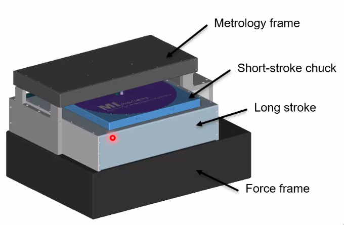
Figure 99: Schematic of the 6dof levitating stage
7.2 Case
More precisely, the goal is to automatically maximize the three eigen-frequencies of the system shown in Figure 100.
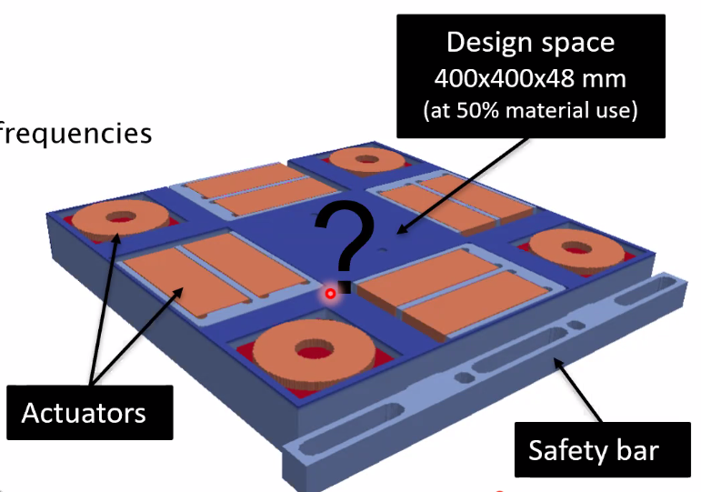
Figure 100: System to be optimized
7.3 Manufacturing process
The manufacturing process must be embedded in the optimization such that the obtained design is producible. The process is shown in Figure 101.
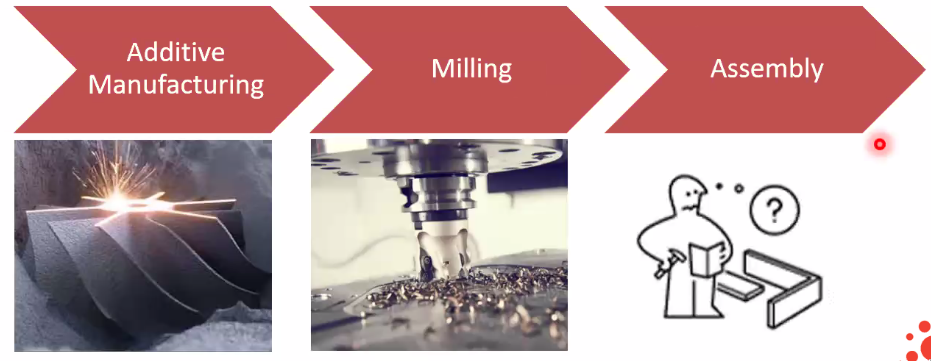
Figure 101: Manufacturing process
7.4 Topology optimization
Problem: for a given volume, maximize the eigen-frequencies of the system.
To do so, the system is discretized into small elements (Figure 102). Then, a Finite Element Analysis is performed to compute the eigen-frequencies of the system. Finally, for each element, the “gradient is computed” and we determine if material should be added or removed.
This is done in 3D. The individual 1mm x 1mm x 1mm elements are shown in Figure 102. The number of elements is 1 million (=> 15 minutes per iteration to compute the 3 eigen-frequencies).
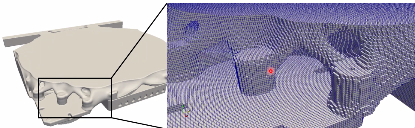
Figure 102: Results of the topology optimization and zoom to see individual elements
7.5 Performance Comparison
The obtained mass and eigen-frequencies of the optimized system and the solid equivalents are compared in Figure 103.
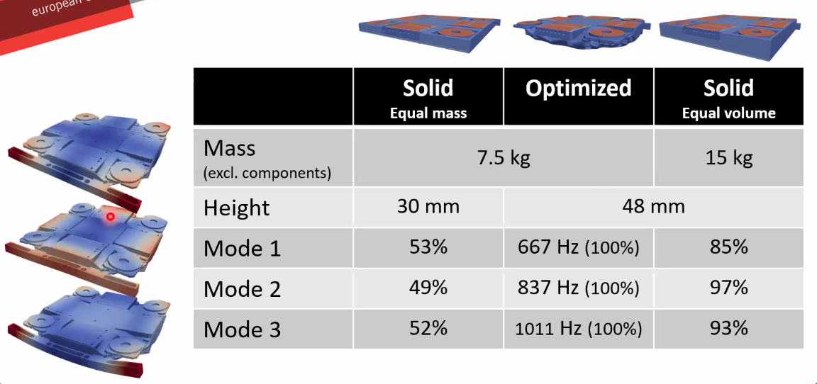
Figure 103: Comparison of the obtained performances
Identification on the realized system shown that the obtained eigen-frequencies are very closed to the estimated ones (Figure 104).
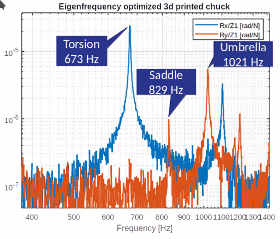
Figure 104: Results very close to simulation (~1% for the eigen frequencies)
7.6 Conclusion
- Increase in performance (~2x) compared to solid designs
- A design is obtained in ~ 1 day
- Practical constraints are incorporated in the optimization
- The method is validated in practice by a demonstrator
8 A multivariable experiment design framework for accurate FRF identification of complex systems @nic_dirkx
8.1 Introduction
Goal: Need for higher quality FRF models that are used to:
- Controller design
- Observer design
- System diagnostics
- Parametric modelling
High quality FRFs requires careful design of excitation \(w\).
Typical experimental identification of the FRFs is shown in Figure 105.
The design trade-off is:
- Maximize input gain to minimize FRF uncertainty
- Bounded signal \(u\) and \(y\) to remain within operating limited (actuator/amplifier power limitations and limited move ranges)
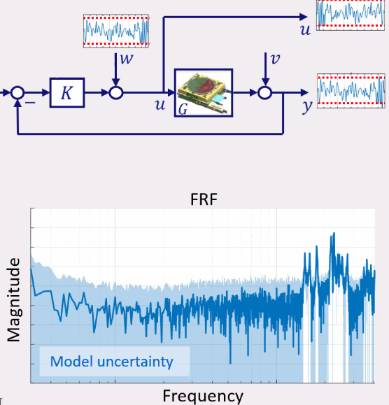
Figure 105: schematic of the identification of the FRF
For SISO systems:
- Only the frequency size of the excitation signal should be optimized
For MIMO systems:
- the gains and directions should be frequency wise optimized
Objective:
- establish optimal experiment design framework that optimize the excitation signal to obtain MIMO FRFs with low uncertainty
8.2 Role of directions and constrains in multivariable excitation design
The classical way to estimate MIMO FRFs is the following:
- First start with one direction and increase the gain until constrains is attained (Figure 106)
- Do the same with the second input
This lead to non-optimal FRFs estimation.
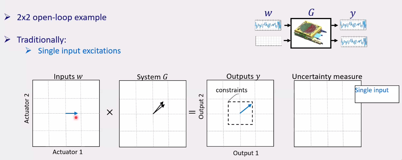
Figure 106: Example of a SISO approach to identify MIMO FRFs
When having a MIMO approach and choosing both the direction and gain of the excitation inputs, we can obtained much better FRFs uncertainty while still fulfilling the constraints (Figure 107).
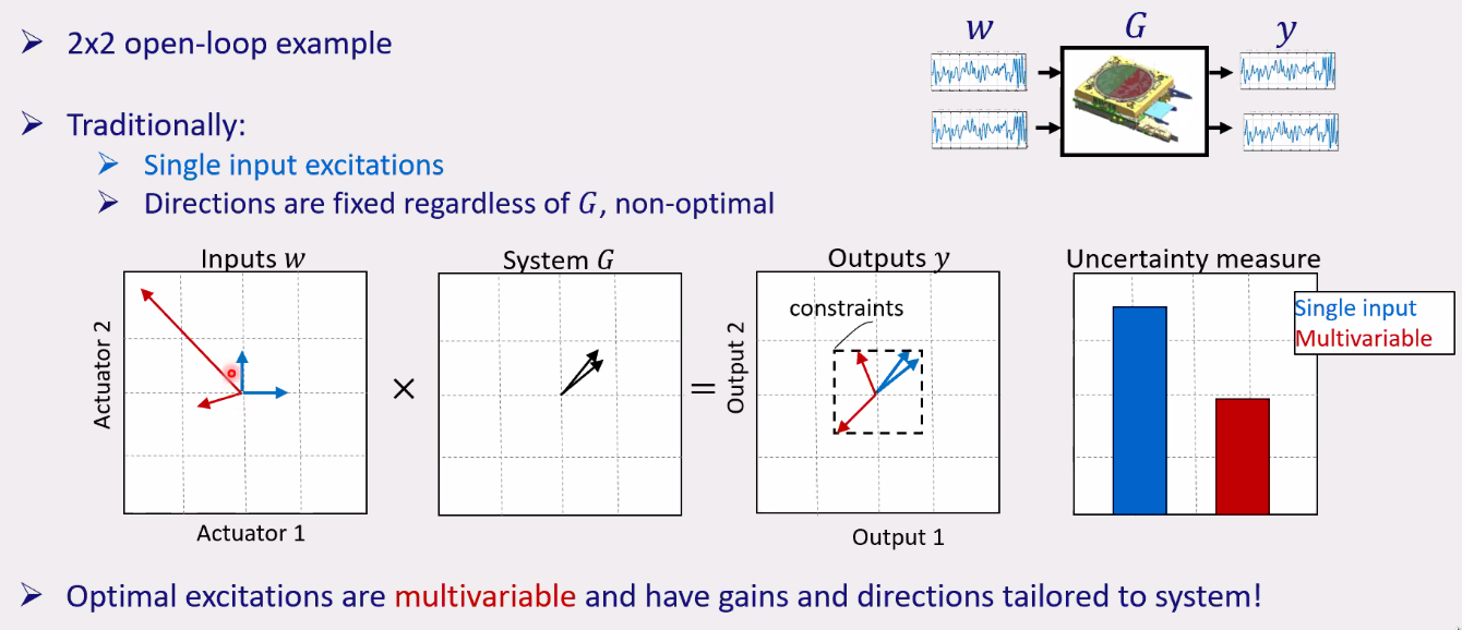
Figure 107: Example of the MIMO approach that gives much better FRFs
8.3 Solving the optimization problem
The optimization problem is to minimize the model uncertainty by choosing the design variables which are the magnitude and direction of the inputs \(w\).
The optimization is a two step process as shown in Figure 108:
- first identification without optimization that allows to have data to run the optimization process
- second identification with optimized input direction and gain
The problem with this optimization problem is that it is not convex in general and has a log of design variables. There is no general methods to solve this problem, a dedicated algorithm is required.
In this work, two algorithms are proposed and not further detailed here.
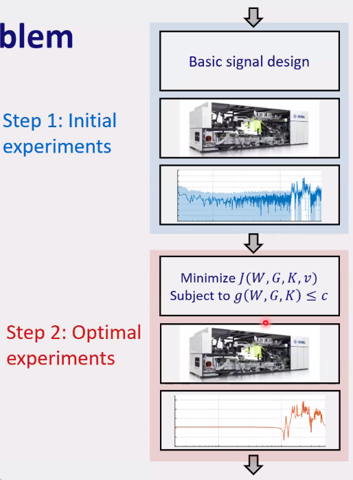
Figure 108: Two step optimization process
8.4 Experimental validation
Experimental identification of a 7x8 MIMO plant was performed in for different cases:
- non optimized SISO approach (grey)
- optimized SISO approach (blue)
- optimized MIMO approach using SSDR (first algorithm proposed) (green)
- optimized MIMO approach using RR (second algorithm proposed) (red)
The obtained FRFs are shown in Figure 109.
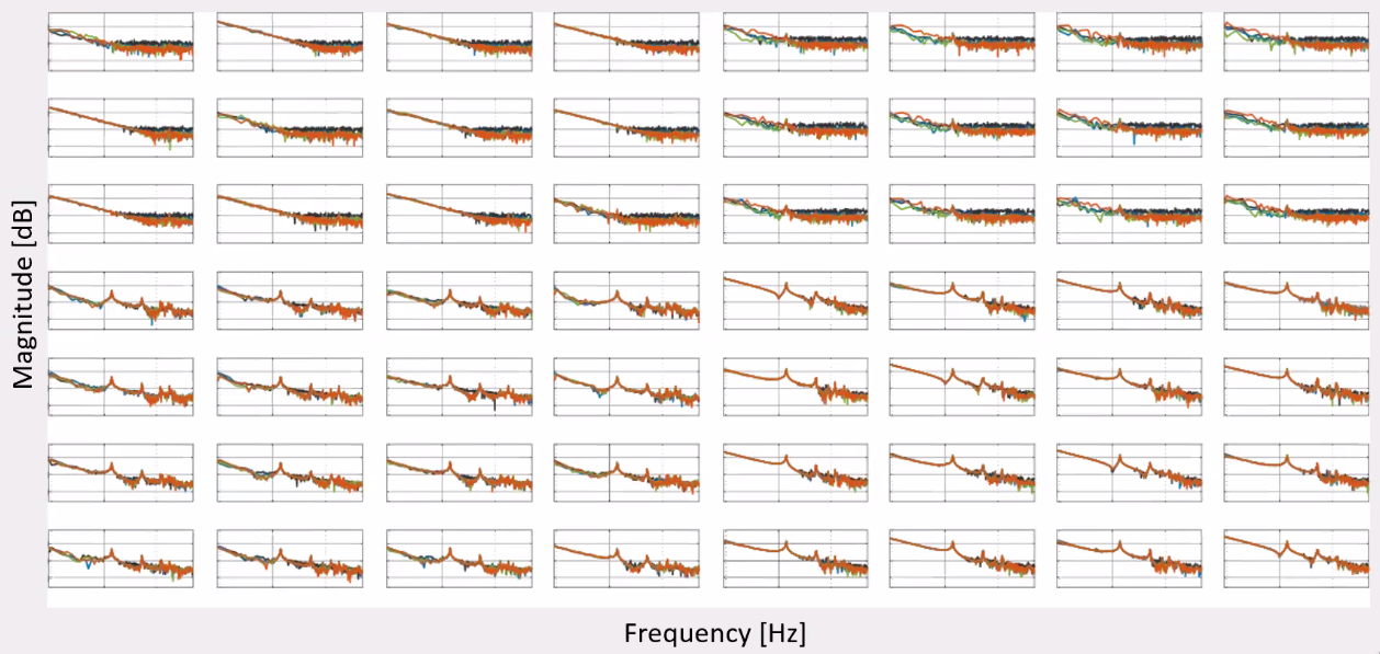
Figure 109: Obtained MIMO FRFs
A comparison of one of the obtained FRFs is shown in Figure 110. It is quite clear that the MIMO approach can give much lower FRF uncertainty. The RR proposed algorithm is giving the best results
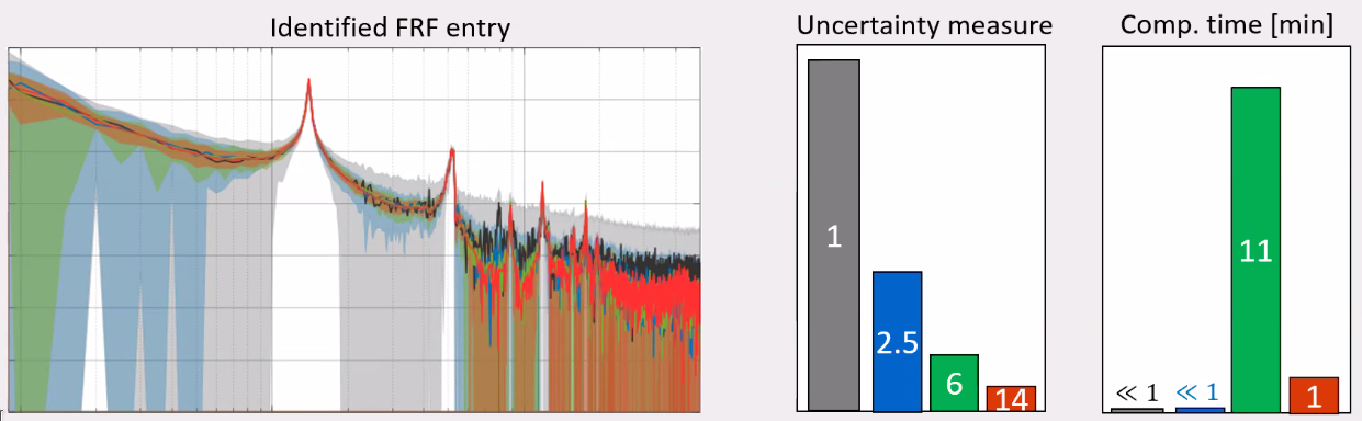
Figure 110: Example of one of the obtained FRF
8.5 Conclusion
- The uncertainty of the obtained FRF are obtained by doing several experimental identification with a deterministic input signal. The FRF are computed multiple times, and the spread of the results at each frequency represents this uncertainty.
- Exploiting directionality in excitation design enables significant FRF quality improvement
- Multivariable design involves hard non-convex optimization problem
- Computationally tractable design framework for large scale MIMO systems established
- Near global optimal quality achieved on wafer stage setup using RR algorithm
9 Reducing control delay times to enhance dynamic stiffness of magnetic bearings @jan_philipp_schmidtmann
9.1 Introduction
This projects focuses on reducing the control delay times of a magnetic bearing shown in Figure 111.
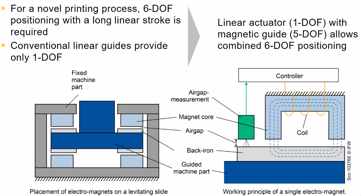
Figure 111: 6 DoF Position System - Concept
Active magnetic bearings are unstable systems and require active control. However, the active control of magnet forces leads to a control delay that limits the performances (stiffness) of the bearing.
9.2 Time Delay Reduction
Typical contributors to the control delay time are shown in Figure 112.
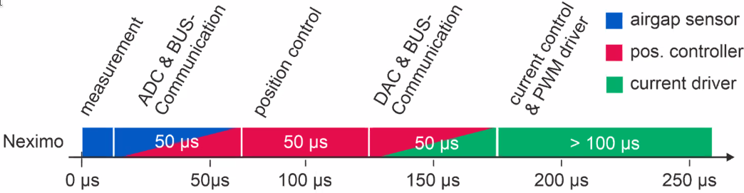
Figure 112: Typical Contributors to control delay time
The reduction of the control time delay will increase the dynamic stiffness of the bearing as well as decrease the effects of external disturbances and hence improve the positioning errors (Figure 113).
The steps to reduce the control delay time are:
- Eliminate BUSS-communication by merging position and current controller
- Reduce cycle time by using rapid prototyping system
- Reduce delay in PWM driver by using high PWM frequencies with SiC driver
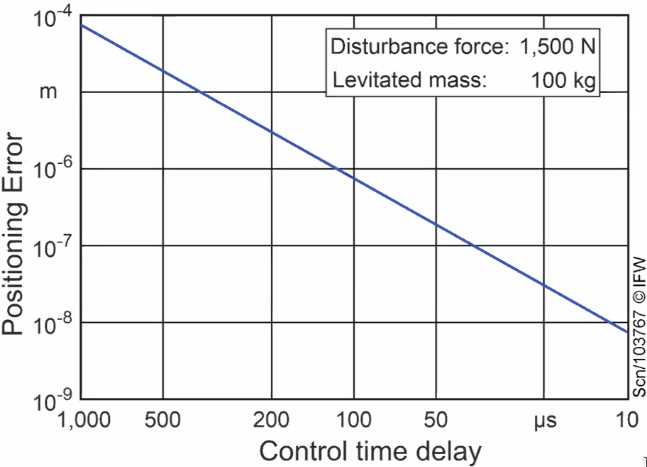
Figure 113: The effect of control delay on stiffness
9.3 Practical Realization
Therefore, the position and current control have been merged into one controller (Figure 114).
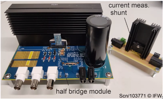
Figure 114: Controller for position and current
A dSpace rapid prototyping system is used for fast position and current control. Characteristics of the used elements are shown in Figure 115.
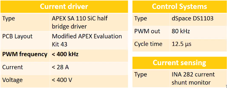
Figure 115: Setup for reduced delay times
9.4 Results
Differences between the previous PWM controller and the new SiC controller are shown in Figure 116. The delay time is almost completely eliminated.
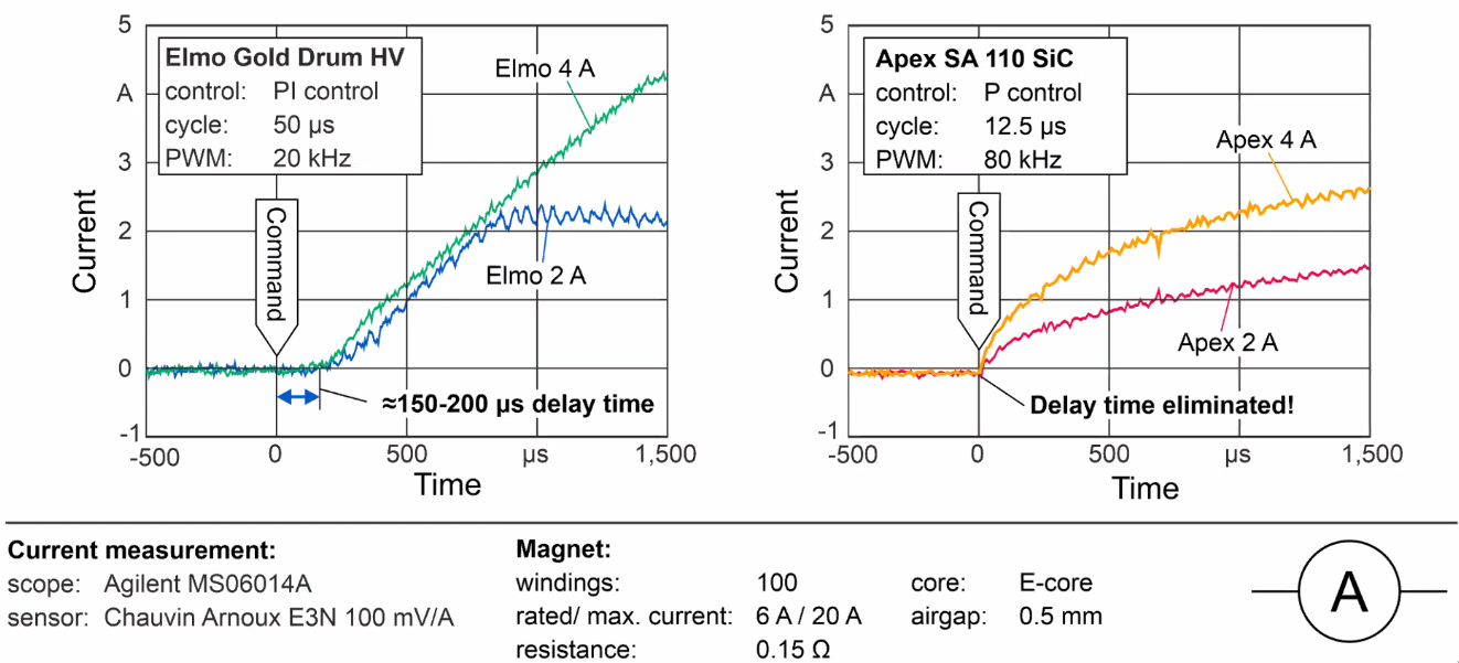
Figure 116: Reduction of delay in PWM Driver
9.5 Conclusion
Due to all the performed modifications, the control delay time could be reduced by 80%. The next steps for this project are shown in Figure 117.
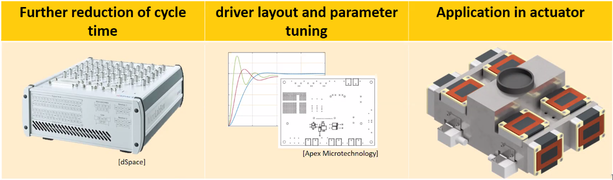
Figure 117: Next Steps
10 Digital twins in control: From fault detection to predictive maintenance in precision mechatronics @koen_classens
10.1 Motivation
Models are usually for the control design part that can be either physical models (FEM, first principle) or data-driven models. However, these models are usually not used after control system is implemented (Figure 118).
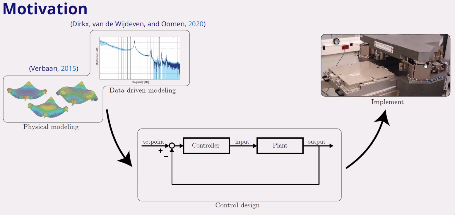
Figure 118: Typical of of models in a mechatronic system
Here, the models are exploited to monitor the system and predict future possible failures in the system. Use models as digital twin for fault detection and Isolation for predictive maintenance in precision mechatronics (Figure 119).
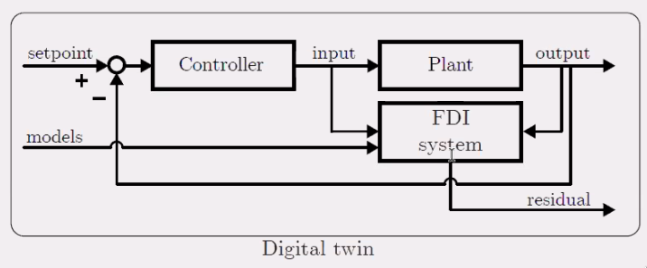
Figure 119: FDI is using the model of the plant
10.2 Predictive Maintenance
Classical maintenance happens when the system is not working anymore as shown in Figure 120.
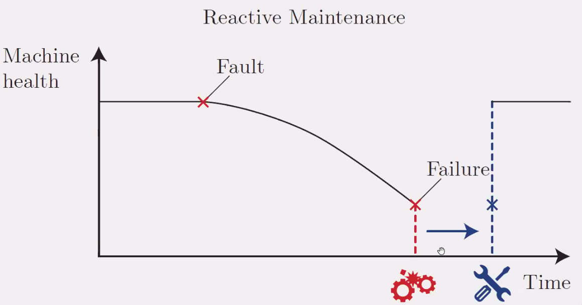
Figure 120: Maintenance done when a failure is appearing
It is possible to perform some preventive maintenance before a failure happens, but this is still not optimal.
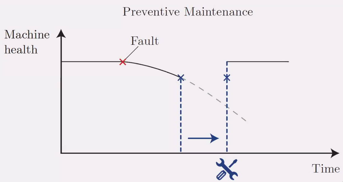
Figure 121: Preventive Maintenance
The idea here is to predict when the failure will happen in order to only do maintenance only when really necessary. This will minimize the down time of the machine.
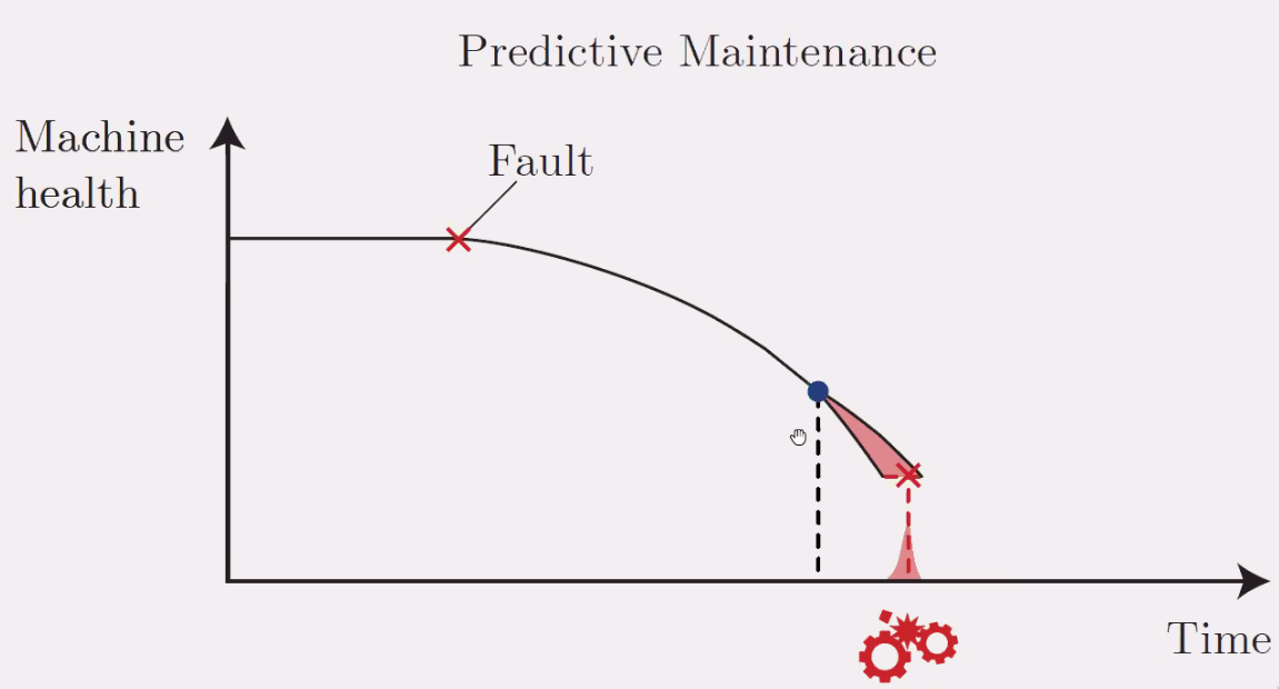
Figure 122: Predictive maintenance
10.3 Objectives
The main objective is to develop a system monitoring approach for precision mechatronic systems, exploiting prior information (models) and integrating posterior information (real-time measured data).
Even though state of the art system monitoring are already in used in aerospace, process industry and automotive, there are few specificity for mechatronic systems:
- Control loops
- Large-scale MIMO systems (interaction)
- Accurate models: Frequency Response Functions
10.4 Null-space based FDI
The goal is to applied a decentralized Fault Detection on the system shown in Figure 123 to detect actuator faults at \(J_1\). This should take into account the control loop, interaction in the system and be FRF based.
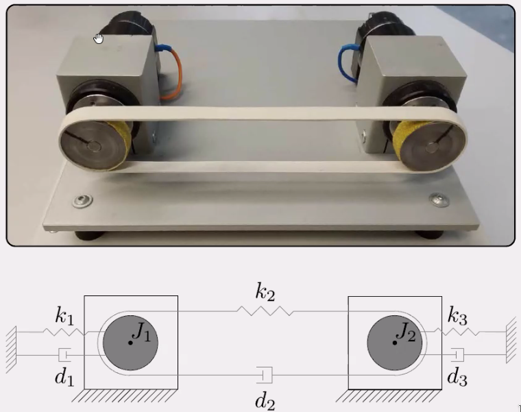
Figure 123: Test System
The architecture to estimate faults in the system is shown in Figure 124. The goal is to design \(Q_u\) and \(Q_y\) such that \(\epsilon\) is a representation of faults in the system.
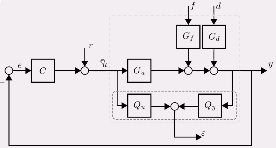
Figure 124: Residual Generator
When a fault happens (Figure 125), the outputs signals are not changing that much (because of feedback), however the system is able to find that there is a problem using the residual \(\epsilon\).
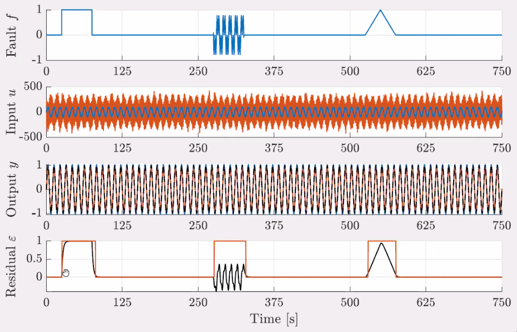
Figure 125: Simulation Results
Procedure:
- Additive faults
- Closed-loop
- Interaction
- start from identification
10.5 Roadmap from fault detection to predictive maintenance
The proposed system can detect faults in the system (Figure 126). This proof of principle should now be applied on industrial systems. Moreover, from the fault detection, predictive maintenance should be performed (Figure 126).
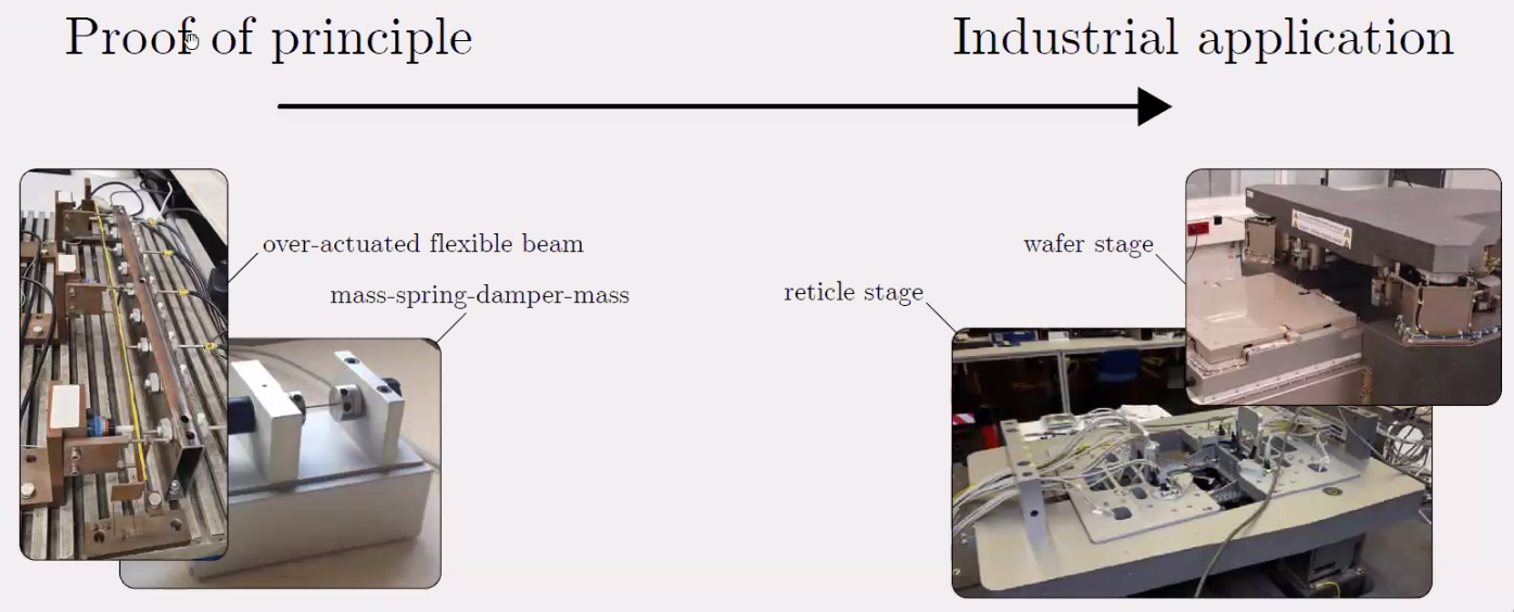
Figure 126: From proof of principle to industrial application
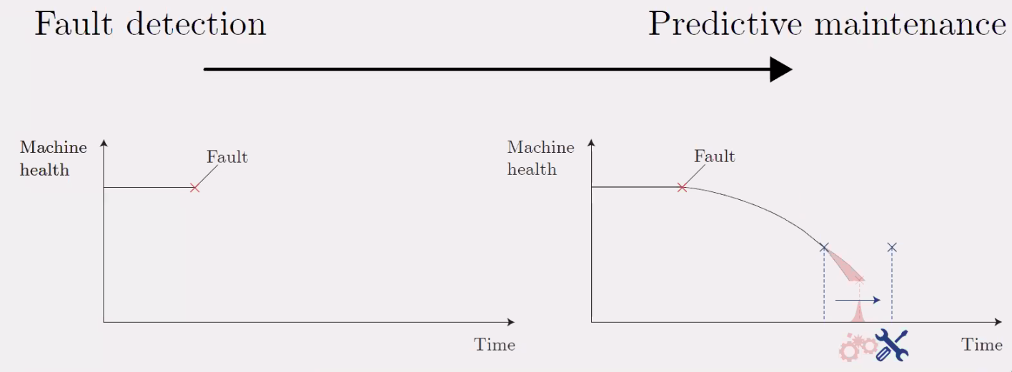
Figure 127: From fault detection to predictive maintenance