Encoder - Test Bench
Table of Contents
This report is also available as a pdf.
In this document, we wish to study the use of an encoder in parallel with an Amplified Piezoelectric Actuator.
The document is divided into the following Sections:
- Section 1: the test-bench used is described
- Section 2: the noise spectral density of the encoder is estimated
- Section 3: the dynamics from the amplified piezoelectric actuator to the encoder measured displacement is identified
1 Experimental Setup
The experimental Setup is schematically represented in Figure 1.
Here are the equipment used in the test bench:
The mass can be vertically moved using the amplified piezoelectric actuator. The displacement of the mass (relative to the mechanical frame) is measured both by the interferometer and by the encoder.
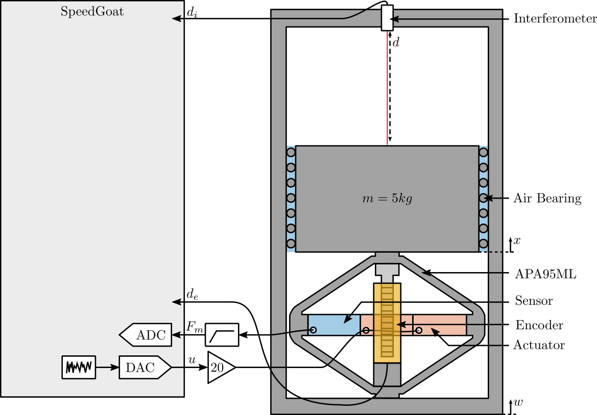
Figure 1: Schematic of the Experiment
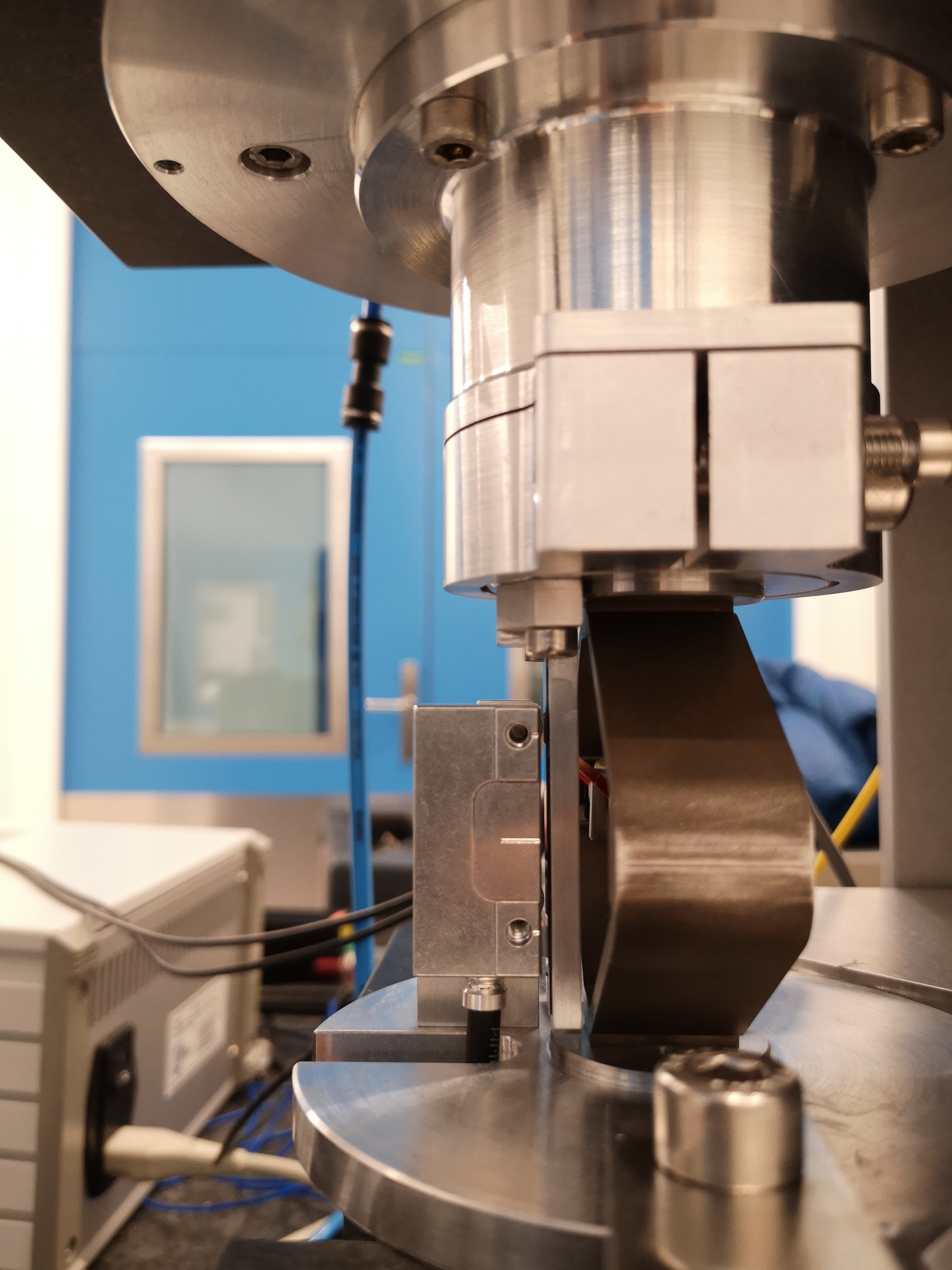
Figure 2: Side View of the encoder
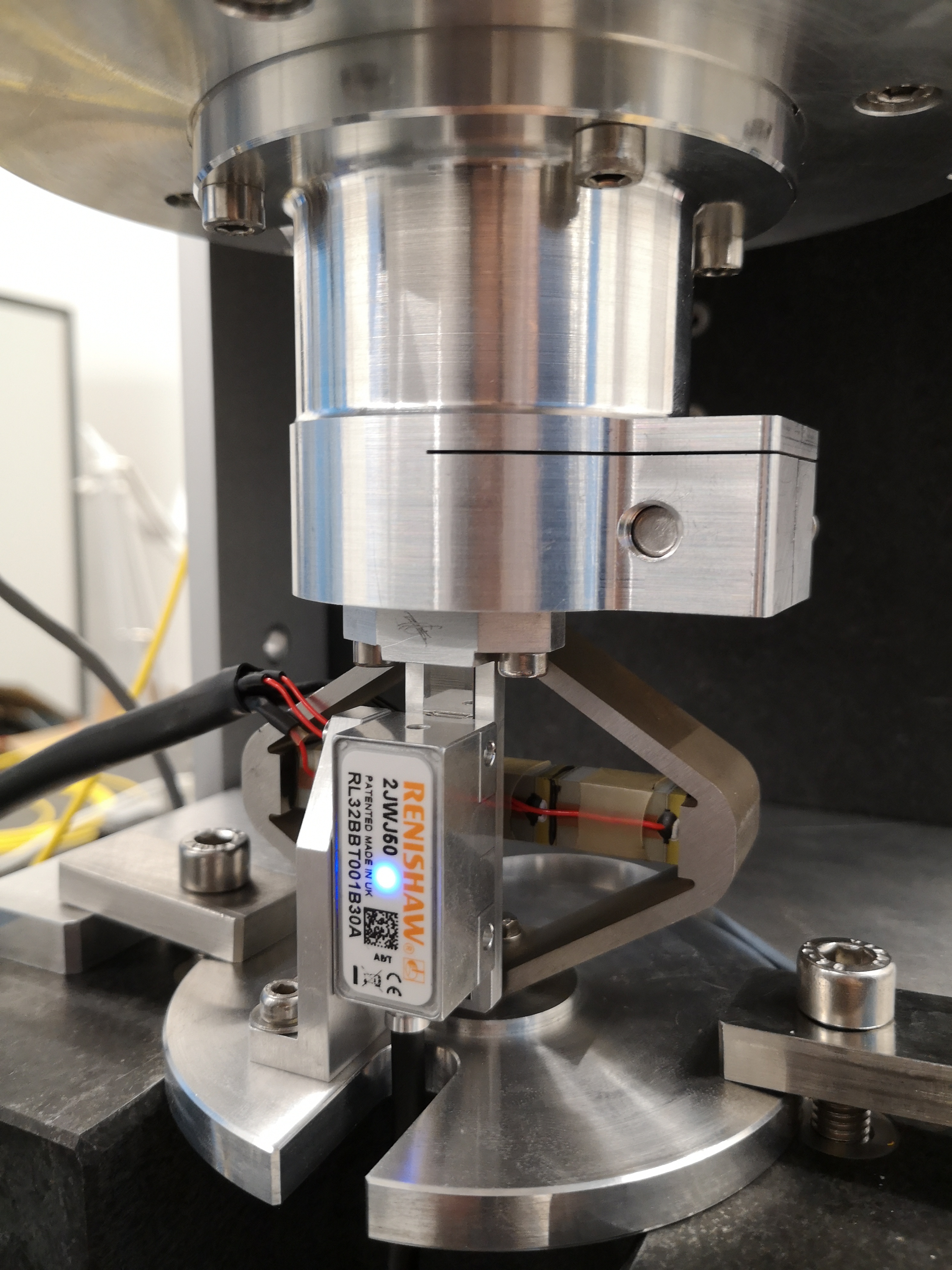
Figure 3: Front View of the encoder
2 Noise Spectral Density of the Encoder
The goal in this section is the estimate the noise of both the encoder and the intereferometer.
The actuator is not excited, thus the relative motion between the mass and the frame is as small as possible. Ideally, a mechanical part would clamp the two together, we here suppose that the APA is still enough to clamp the two together.
2.1 Load Data
The measurement data are loaded and the offset are removed using the detrend command.
load('int_enc_huddle_test.mat', 'interferometer', 'encoder', 't');
  interferometer = detrend(interferometer, 0);
  encoder = detrend(encoder, 0);
2.2 Time Domain Results
The measurement of both the encoder and interferometer are shown in Figure 4.
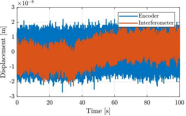
Figure 4: Huddle test - Time domain signals
The raw signals are filtered with a Low Pass filter (defined below) such that we can see the low frequency motion (Figure 5).
G_lpf = 1/(1 + s/2/pi/10);
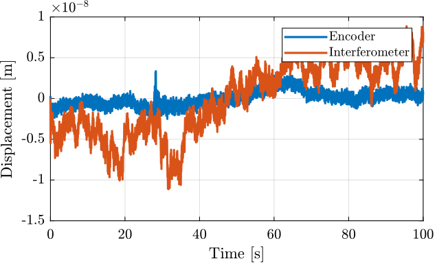
Figure 5: Huddle test - Time domain signals filtered with a LPF at 10Hz
2.3 Frequency Domain Noise
The noise of the measurement (supposing there is no motion) is now translated in the frequency domain by computed the Amplitude Spectral Density.
  Ts = 1e-4;
  win = hann(ceil(10/Ts));

  [p_i, f] = pwelch(interferometer, win, [], [], 1/Ts);
  [p_e, ~] = pwelch(encoder,        win, [], [], 1/Ts);
The comparison of the ASD of the encoder and interferometer are shown in Figure 6.
It is clear that although the encoder exhibit higher frequency noise, is it more stable at low frequency as the length of the beam path in the air is much smaller and thus changed of temperature/pressure/humity of the air has much smaller effect on the measured displacement.
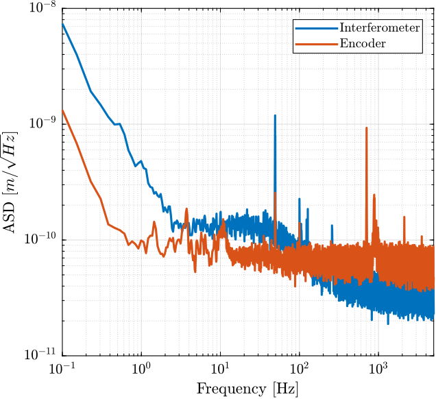
Figure 6: Amplitude Spectral Density of the signals during the Huddle test
3 Dynamics from Actuator to Encoder
3.1 Load Data
As usual, the measurement data are loaded.
load('int_enc_id_noise_bis.mat', 'interferometer', 'encoder', 'u', 't');
The first 0.1 seconds are removed as it corresponds to transient behavior.
  interferometer = interferometer(t>0.1);
  encoder = encoder(t>0.1);
  u = u(t>0.1);
  t = t(t>0.1);
Finally the offset are removed using the detrend command.
  interferometer = detrend(interferometer, 0);
  encoder = detrend(encoder, 0);
  u = detrend(u, 0);
3.2 Excitation and Measured Signals
The excitation signal is a white noise filtered by a low pass filter to not excite too much the high frequency modes.
The excitation signal is shown in Figure 7.
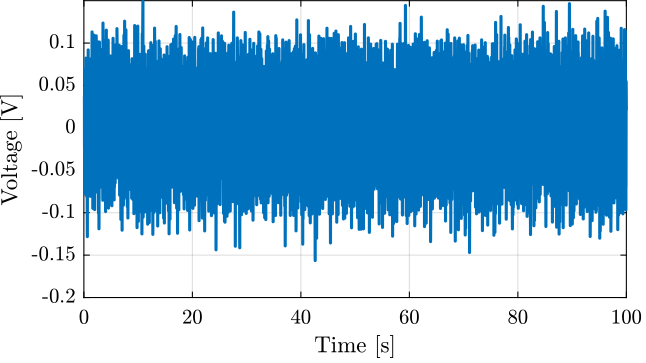
Figure 7: Excitation Voltage
The measured motion by the interferometer and encoder is shown in Figure
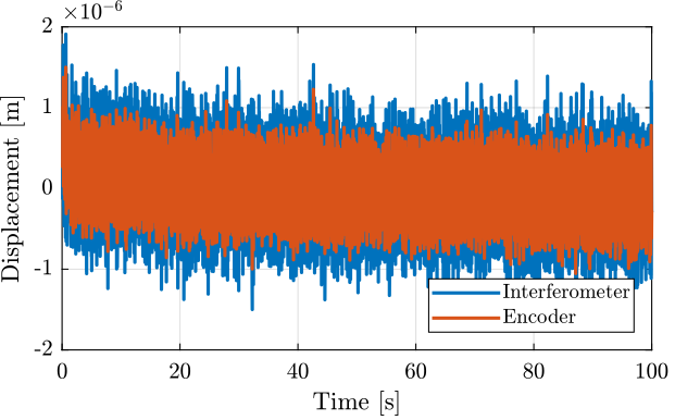
Figure 8: Measured displacement by the encoder and interferometer
3.3 Identification
Now the dynamics from the voltage sent to the voltage amplitude driving the APA95ML to the measured displacement by both the encoder and interferometer are computed.
  Ts = 1e-4; % Sampling Time [s]
  win = hann(ceil(10/Ts));

  [tf_i_est, f] = tfestimate(u, interferometer, win, [], [], 1/Ts);
  [co_i_est, ~] = mscohere(u, interferometer, win, [], [], 1/Ts);

  [tf_e_est, ~] = tfestimate(u, encoder, win, [], [], 1/Ts);
  [co_e_est, ~] = mscohere(u, encoder, win, [], [], 1/Ts);
The obtained coherence is shown in Figure 9. It is shown that the identification is good until 500Hz for the interferometer and until 1kHz for the encoder.
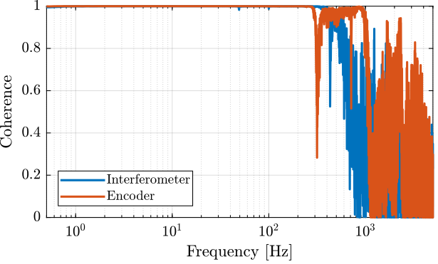
Figure 9: Obtained coherence for both the encoder and interferometer
The compared dynamics as measured by the intereferometer and encoder are shown in Figure 10.
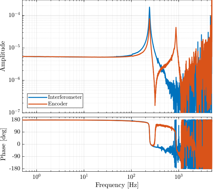
Figure 10: Obtained dynamics from actuator voltage to displacement as measured by the interferometer and by the encoder
The second resonance at around 900Hz most likely corresponds to the resonance of either the ruler support or the head support.