ESRF Double Crystal Monochromator - Compensating Repeatable Positioning Errors of Fast Jacks
Table of Contents
- 1. Hardware and Software Implementation
- 2. Initial and proposed LUT computations
- 3. LUT creation from experimental data
- 3.1. Load Data
- 3.2. IcePAP generated Steps
- 3.3. Bragg and Fast Jack Velocities
- 3.4. Bragg Angle Errors / Delays
- 3.5. Errors in the Frame of the Crystals
- 3.6. Errors in the Frame of the Fast Jacks
- 3.7. Analysis of the obtained error
- 3.8. Filtering of Data
- 3.9. LUT creation
- 3.10. Cubic Interpolation of the LUT
- 4. Position Repeatability
- 5. LUT Software Implementation
- 6. Optimal Trajectory
- 7. Constant Fast Jack velocity
- 8. Effect of the number of points in the trajectory in mode B
- 9. LUT for energy scans (XANES)
- 10. Merge LUT
This report is also available as a pdf.
This document summarizes the studies done on the compensation of repeatable errors of the Fast Jacks.
Each Fast Jack is composed of one stepper motor directly driving (i.e. without any reducer) a ball screw with a pitch of 1mm (i.e. 1 stepper motor turn makes a 1mm linear motion).
When scanning using the fast jack without any sort of control (i.e. in mode A), rather large positioning errors can be measured by the interferometers.
Some of these errors are repeatable while other are not repeatable (see Section 4).
It is here studied how to measure these repeatable positioning errors and how to compensate them using a Lookup Table (LUT).
This functioning mode is called mode B.
Then there is a piezoelectric stack in series with the fast-jack which is working in closed-loop with the interferometer signals and that is used to compensate the remaining (mostly non-repeatable) errors induced by the stepper motor and other disturbances.
This is called mode C.
The compensation of repeatable errors using the Lookup Tables has several goals:
- Reducing the positioning errors below the stroke of the piezoelectric stack actuator. Otherwise the stroke of the piezoelectric stack in mode C (feedback control) could be too small and errors cannot be further controlled.
- Reducing the errors above the bandwidth of the feedback controller. The bandwidth of the feedback controller is limited by the mechanical behavior of the DCM, and therefore vibrations outside this bandwidth can only be compensated using calibration / lookup tables.
The general procedure to compute and use the LUT is shown in Figure 1.
Note that there is some exchange of information between each step indicated by the arrow and some .dat file containing the data.
It can separated into four main steps:
- Perform a scan in mode A in order to properly measure the Fast Jack motion errors. The scan should be done in such a way that the motion errors of the Fast Jack can be separated from the other disturbances and non-repeatable errors by the use of filtering. This is the subject of Sections 6 and 7
- Compute the LUT from the measured errors.
For each Fast Jack, the LUT associates the wanted position with the corresponding IcePAP step at which the Fast Jack is effectively at the correct position (as measured during the previous scan).
This is discussed in Section 2 and the software implementation is described in Section 5.
The LUT data is stored in a
lut.datfile and can be further loaded in the next step. - Generate a trajectory. The trajectory links several motors for synchronization (mainly bragg with fast jacks). The LUT data is included in this trajectory such that the measured repeatable errors that are included in the LUT are compensated. This is discussed in Section 8.
- Make a scan in mode B. The IcePAP is moving all motors in a synchronized way and tries to follow the trajectory data with included compensation of repeatable errors.
The Hardware and Software setup used for the measurement and tests of the lookup table is described in Section 1.
For each of these steps, several problems can lead to inaccuracies in the computed LUT and trajectory which will result in non optimal compensation of repeatable errors during a scan in mode B. In order to have the best possible mode B positioning accuracy, each of these problems are studied in this document.
A comparison between the way the LUT was built before December 2021 and after is performed in Section 2. Complete process from measurement of Fast-Jack errors to the tests in mode B is described in Section 3.
As the DCM will be used for X-ray absorption techniques such as XANES, recommended scan parameters are given in Section 9.
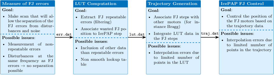
Figure 1: Overview of the process to make the LUT and associated possible issues.
1. Hardware and Software Implementation
In this section, a brief description of the experimental setup required to computed the Lookup Tables is given (Section 1.2).
It is important also to see how the trajectories and Lookup Tables are computed and implemented in terms of software in order to understand the possible limitations. This is described in Section 1.1.
1.1. Measurement setup
In order to measure the errors induced by the fast jacks, scans have to be made, and the following signals have to be measured simultaneously:
- The wanted fast jack position: step sent by the IcePAP
- The actual (measured) position
The experimental setup is schematically shown in Figure 2.
The procedure is the following:
- A Bragg angle trajectory \(\theta\) is generated from Bliss and loaded in the IcePAP as a kind of lookup table. This lookup table is only used to synchronize all the motors, and no compensation of errors are implemented.
- The IcePAP generates some steps \([u_{u_r},\ u_{u_h},\ u_{d}]\) that are sent to the fast jacks.
- The motion of the crystals \([d_z,\ r_y,\ r_x]\) is measured with the interferometers. The transformation from interferometers values to position and orientation errors of crystals is performed inside the Speedgoat.
- Finally, the corresponding motion \([d_{u_r},\ r_{u_h},\ r_d]\) of the each fast jack is computed afterwards in BLISS.
In order to create the LUT, the measured motion of the fast jacks \([d_{u_r},\ r_{u_h},\ r_d]\) and the IcePAP steps \([u_{u_r},\ u_{u_h},\ u_{d}]\) have to be measured simultaneously.
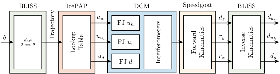
Figure 2: Block diagram of the experiment to create the Lookup Table
1.2. LUT Implementation
The computation of the LUT consists of generating an array with 4 columns.
The first column corresponds to the position (in mm) where it is wanted to position the Fast Jack.
The remaining three columns are corresponding (for each motor: fjpur, fjpuh and fjpd) to the position (i.e. step) where the IcePAP should position the motors such that the real position is corresponding to the first column.
This array lut.dat can have as many lines as wanted.
In BLISS, it is specified where the LUT is stored using the following command:
dcm.lut.load(data_file="lut.dat", data_dir="directory_where_lut_are_stored")
Then, to use the LUT, a trajectory has to be loaded with the use_lut=True parameter:
dcm.trajectory.load_bragg(12, 18, 1000, use_lut=True)
To perform the trajectory (synchronization of several motors), a “trajectory motor” is used in the IcePAP.
This motor is virtual and is used to synchronize the following motors: mbrag, msafe, mcoil, fjsur, fjsuh and fjsd.
To specify how to do the trajectory, an array with 7 columns is used.
The first column corresponds to the “trajectory motor” (i.e. Bragg, FJS, Energy, …).
The remaining 6 columns are the 6 real motors that have to be synchronized.
Values are computed based on theoretical positions.
The lines of this array are separated with an constant fjs increment which is specified by the parameter 1000 when loading the trajectory.
The parameter 1000 indicates that the trajectory should contains 1000 points every millimeter of the Fast Jack motion.
In that case, the trajectory will be specific for every micrometer of fast jack motion.
Note that the loaded points of the trajectory are always with constant Fast Jack motion increment even though the trajectory is made over Bragg angle or energy.
Then, if use_lut=True is used, the LUT data will be integrated in the motor trajectory by modifying the columns corresponding to the fjsur, fjsuh and fjsd motors.
For every point in the trajectory:
- the data in the LUT corresponding to the wanted position of the fast-jack is found
- a linear interpolation between the two adjacent points is performed, and the result is loaded in the array
Then, when performing a trajectory, the IcePAP will use the loaded data (including the LUT information) to control the position of each motor. Spline interpolation is performed between the specified points in the LUT.
Therefore, several errors can be introduced even though the LUT is computed from perfect data:
- Linear interpolation of the LUT when computing the trajectory points can result in large errors if not enough points are used in the LUT
- Spline interpolation in the IcePAP can introduce errors
2. Initial and proposed LUT computations
2.1. Patterns in the Fast Jack motion errors
In order to understand what should be the “sampling distance” for the lookup table of the stepper motor, we have to analyze the displacement errors induced by the stepper motor.
Let’s load the measurements of one bragg angle scan without any LUT.
%% Load Data of the new LUT method
ol_bragg = (pi/180)*1e-5*double(h5read('Qutools_test_0001.h5','/33.1/instrument/trajmot/data')); % Bragg angle [rad]
ol_dzw   = 10.5e-3./(2*cos(ol_bragg)); % Wanted distance between crystals [m]

ol_dz    = 1e-9*double(h5read('Qutools_test_0001.h5','/33.1/instrument/xtal_111_dz_filter/data'));  % Dz distance between crystals [m]
ol_dry   = 1e-9*double(h5read('Qutools_test_0001.h5','/33.1/instrument/xtal_111_dry_filter/data')); % Ry [rad]
ol_drx   = 1e-9*double(h5read('Qutools_test_0001.h5','/33.1/instrument/xtal_111_drx_filter/data')); % Rx [rad]

ol_t = 1e-6*double(h5read('Qutools_test_0001.h5','/33.1/instrument/time/data')); % Time [s]

ol_ddz   = ol_dzw-ol_dz; % Distance Error between crystals [m]
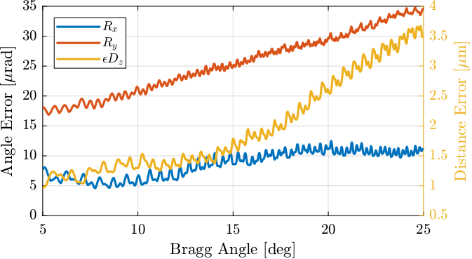
Figure 3: Orientation and Distance error of the Crystal measured by the interferometers
Now let’s convert the errors from the frame of the crystal to the frame of the fast jacks (inverse kinematics problem) using the Jacobian matrix.
%% Compute Fast Jack position errors
% Jacobian matrix for Fast Jacks and 111 crystal
J_a_111 = [1,  0.14, -0.1525
           1,  0.14,  0.0675
           1, -0.14,  0.0425];

ol_de_111 = [ol_ddz'; ol_dry'; ol_drx'];

% Fast Jack position errors
ol_de_fj = J_a_111*ol_de_111;

ol_fj_ur = ol_de_fj(1,:);
ol_fj_uh = ol_de_fj(2,:);
ol_fj_d  = ol_de_fj(3,:);
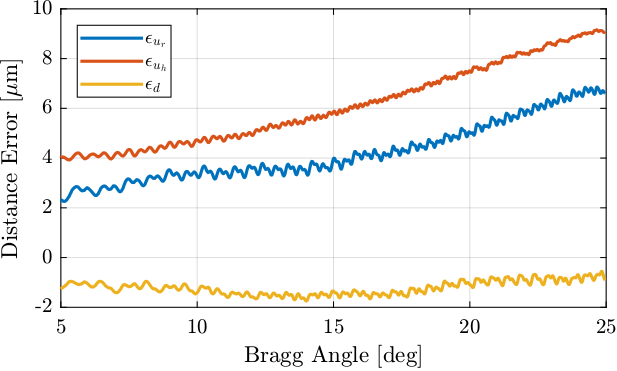
Figure 4: Estimated motion errors of the fast jacks during the scan
Let’s now identify this pattern as a function of the fast-jack position.
As we want to done frequency Fourier transform, we need to have uniform sampling along the fast jack position.
To do so, the function resample is used.
Xs = 0.1e-6; % Sampling Distance [m]

%% Re-sampled data with uniform spacing [m]
ol_fj_ur_u = resample(ol_fj_ur, ol_dzw, 1/Xs);
ol_fj_uh_u = resample(ol_fj_uh, ol_dzw, 1/Xs);
ol_fj_d_u  = resample(ol_fj_d,  ol_dzw, 1/Xs);

ol_fj_u = Xs*[1:length(ol_fj_ur_u)]; % Sampled Jack Position
The result is shown in Figure 5.
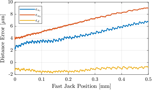
Figure 5: Position error of fast jacks as a function of the fast jack motion
Let’s now perform a Power Spectral Analysis of the measured displacement errors of the Fast Jack.
% Hanning Windows with 250um width
win = hanning(floor(400e-6/Xs));

% Power Spectral Density [m2/(1/m)]
[S_fj_ur, f] = pwelch(ol_fj_ur_u-mean(ol_fj_ur_u), win, 0, [], 1/Xs);
[S_fj_uh, ~] = pwelch(ol_fj_uh_u-mean(ol_fj_uh_u), win, 0, [], 1/Xs);
[S_fj_d,  ~] = pwelch(ol_fj_d_u -mean(ol_fj_d_u ),  win, 0, [], 1/Xs);
As shown in Figure 6, we can see a fundamental “reciprocal length” of \(5 \cdot 10^4\,[1/m]\) and its harmonics. This corresponds to a length of \(\frac{1}{5\cdot 10^4} = 20\,[\mu m]\).
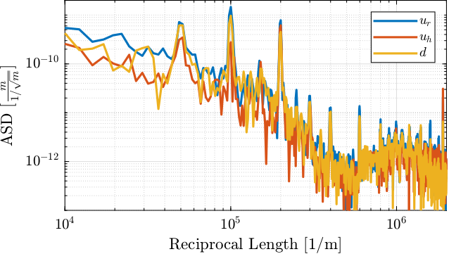
Figure 6: Spectral content of the error as a function of the reciprocal length
Instead of looking at that as a function of the reciprocal length, we can look at it as a function of the spectral distance (Figure 7).
We see that the errors have a pattern with “spectral distances” equal to \(5\,[\mu m]\), \(10\,[\mu m]\), \(20\,[\mu m]\) and smaller harmonics.
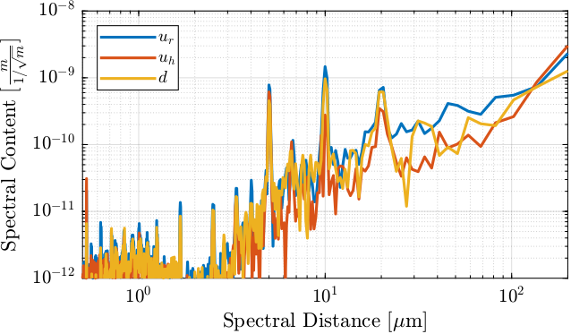
Figure 7: Spectral content of the error as a function of the spectral distance
Let’s try to understand these results. One turn of the stepper motor corresponds to a vertical motion of 1mm. The stepper motor has 50 pairs of poles, therefore one pair of pole corresponds to a motion of \(20\,[\mu m]\) which is the fundamental “spectral distance” we observe.
CPS_ur = flip(-cumtrapz(flip(f), flip(S_fj_ur)));
CPS_uh = flip(-cumtrapz(flip(f), flip(S_fj_uh)));
CPS_d  = flip(-cumtrapz(flip(f), flip(S_fj_d)));
From Figure 8, we can see that if the motion errors with a period of \(5\,[\mu m]\) and \(10\,[\mu m]\) can be dealt with the lookup table, this will reduce a lot the positioning errors of the fast jack.
%% Cumulative Spectrum
figure;
hold on;
plot(1e6./f, sqrt(CPS_ur), 'DisplayName', '$u_r$');
plot(1e6./f, sqrt(CPS_uh), 'DisplayName', '$u_j$');
plot(1e6./f, sqrt(CPS_d),  'DisplayName', '$d$');
hold off;
set(gca, 'xscale', 'log'); set(gca, 'yscale', 'log');
xlabel('Spectral Distance [$\mu m$]'); ylabel('Cumulative Spectrum [$m$]')
xlim([1, 500]); ylim([1e-9, 1e-5]);
legend('location', 'northwest');
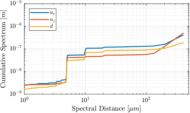
Figure 8: Cumulative spectrum from small spectral distances to large spectral distances
2.2. Experimental Data - Current Method
The current used method is an iterative one.
%% Load Experimental Data
ol_bragg    = double(h5read('first_beam_0001.h5','/31.1/instrument/trajmot/data'));
ol_drx      = h5read('first_beam_0001.h5','/31.1/instrument/xtal_111_drx_filter/data');

lut_1_bragg = double(h5read('first_beam_0001.h5','/32.1/instrument/trajmot/data'));
lut_1_drx   = h5read('first_beam_0001.h5','/32.1/instrument/xtal_111_drx_filter/data');

lut_2_bragg = double(h5read('first_beam_0001.h5','/33.1/instrument/trajmot/data'));
lut_2_drx   = h5read('first_beam_0001.h5','/33.1/instrument/xtal_111_drx_filter/data');

lut_3_bragg = double(h5read('first_beam_0001.h5','/34.1/instrument/trajmot/data'));
lut_3_drx   = h5read('first_beam_0001.h5','/34.1/instrument/xtal_111_drx_filter/data');

lut_4_bragg = double(h5read('first_beam_0001.h5','/36.1/instrument/trajmot/data'));
lut_4_drx   = h5read('first_beam_0001.h5','/36.1/instrument/xtal_111_drx_filter/data');
The relative orientation of the two 111 mirrors in the \(x\) directions are compared in Figure 9 for several iterations.
We can see that after the first iteration, the orientation error has an opposite sign as for the case without LUT.
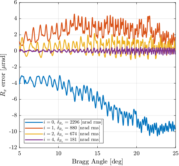
Figure 9: \(R_x\) error with the current LUT method
2.3. Simulation
In this section, we suppose that we are in the frame of one fast jack (all transformations are already done), and we wish to create a LUT for one fast jack.
Let’s say with make a Bragg angle scan between 10deg and 60deg during 100s.
Fs = 10e3; % Sample Frequency [Hz]
t = 0:1/Fs:10; % Time vector [s]
theta = linspace(10, 40, length(t)); % Bragg Angle [deg]
The IcePAP steps are following the theoretical formula:
\begin{equation} d_z = \frac{d_{\text{off}}}{2 \cos \theta} \end{equation}with \(\theta\) the bragg angle and \(d_{\text{off}} = 10\,mm\).
The motion to follow is then:
perfect_motion = 10e-3./(2*cos(theta*pi/180)); % Perfect motion [m]
And the IcePAP is generated those steps:
icepap_steps = perfect_motion; % IcePAP steps measured by Speedgoat [m]
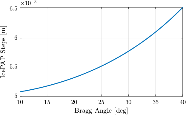
Figure 10: IcePAP Steps as a function of the Bragg Angle
Then, we are measuring the motion of the Fast Jack using the Interferometer. The motion error is larger than in reality to be angle to see it more easily.
motion_error = 100e-6*sin(2*pi*perfect_motion/1e-3); % Error motion [m]

measured_motion = perfect_motion + motion_error; % Measured motion of the Fast Jack [m]
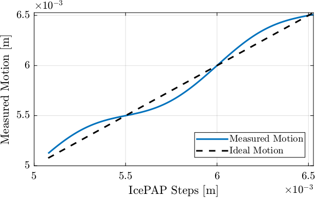
Figure 11: Measured motion as a function of the IcePAP Steps
Let’s now compute the lookup table. For each micrometer of the IcePAP step, another step is associated that correspond to a position closer to the wanted position.
%% Get range for the LUT
% We correct only in the range of tested/measured motion
lut_range = round(1e6*min(icepap_steps)):round(1e6*max(icepap_steps)); % IcePAP steps [um]

%% Initialize the LUT
lut = zeros(size(lut_range));

%% For each um in this range
for i = 1:length(lut_range)
    % Get points indices where the measured motion is closed to the wanted one
    close_points = measured_motion > 1e-6*lut_range(i) - 500e-9 & measured_motion < 1e-6*lut_range(i) + 500e-9;
    % Get the corresponding closest IcePAP step
    lut(i) = round(1e6*mean(icepap_steps(close_points))); % [um]
end
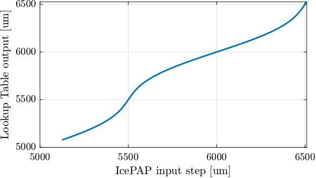
Figure 12: Generated Lookup Table
The current LUT implementation is the following:
motion_error_lut = zeros(size(lut_range));
for i = 1:length(lut_range)
    % Get points indices where the icepap step is close to the wanted one
    close_points = icepap_steps > 1e-6*lut_range(i) - 500e-9 & icepap_steps < 1e-6*lut_range(i) + 500e-9;
    % Get the corresponding motion error
    motion_error_lut(i) = lut_range(i) + (lut_range(i) - round(1e6*mean(measured_motion(close_points)))); % [um]
end
Let’s compare the two Lookup Table in Figure 13.
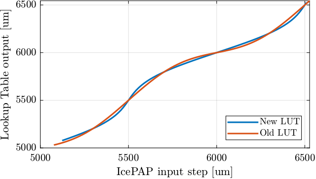
Figure 13: Comparison of the two lookup tables
If we plot the “corrected steps” for all steps for both methods, we clearly see the difference (Figure 14).
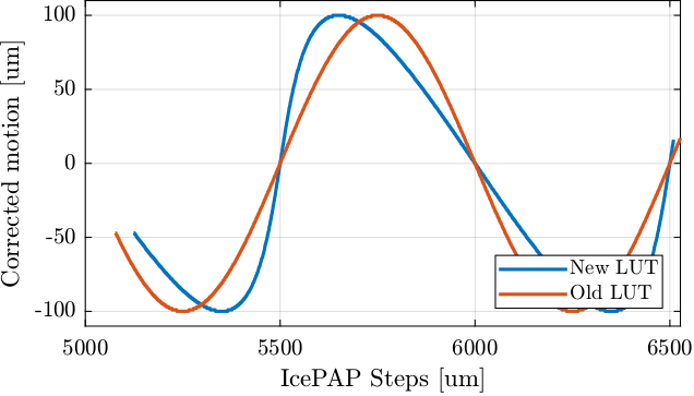
Figure 14: LUT correction and motion error as a function of the IcePAP steps
Let’s now implement both LUT to see which implementation is correct.
motion_new = zeros(size(icepap_steps_output_new));
motion_old = zeros(size(icepap_steps_output_old));

for i = 1:length(icepap_steps_output_new)
    [~, i_step] = min(abs(icepap_steps_output_new(i) - 1e6*icepap_steps));
    motion_new(i) = measured_motion(i_step);

    [~, i_step] = min(abs(icepap_steps_output_old(i) - 1e6*icepap_steps));
    motion_old(i) = measured_motion(i_step);
end
The output motion with both LUT are shown in Figure 15. It is confirmed that the new LUT is the correct one. Also, it is interesting to note that the old LUT gives an output motion that is above the ideal one, as was seen during the experiments.
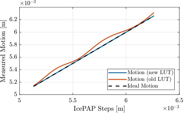
Figure 15: Comparison of the obtained motion with new and old LUT
2.4. Experimental Data - Proposed method (BLISS first implementation)
The new proposed method has been implemented and tested.
The result is shown in Figure 16. After only one iteration, the result is close to the previous method.
%% Load Data of the new LUT method
ol_new_bragg = double(h5read('Qutools_test_0001.h5','/33.1/instrument/trajmot/data'));
ol_new_drx   = h5read('Qutools_test_0001.h5','/33.1/instrument/xtal_111_drx_filter/data');

lut_new_bragg = double(h5read('Qutools_test_0001.h5','/34.1/instrument/trajmot/data'));
lut_new_drx   = h5read('Qutools_test_0001.h5','/34.1/instrument/xtal_111_drx_filter/data');
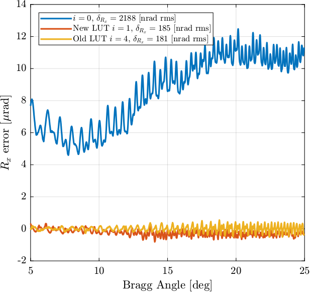
Figure 16: Comparison of the \(R_x\) error for the current LUT method and the proposed one
If we zoom on the 20deg to 25deg bragg angles, we can see that the new method has much less “periodic errors” as compared to the previous one which shows some patterns.
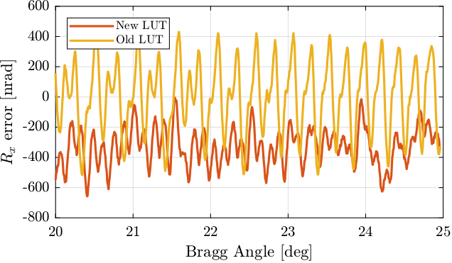
Figure 17: Comparison of the residual motion after old LUT and new LUT
2.5. Comparison of the errors in the reciprocal length space
%% Load Data of the new LUT method
ol_bragg = (pi/180)*1e-5*double(h5read('Qutools_test_0001.h5','/33.1/instrument/trajmot/data'));
ol_dz    = 1e-9*double(h5read('Qutools_test_0001.h5','/33.1/instrument/xtal_111_dz_filter/data'));
ol_dry   = 1e-9*double(h5read('Qutools_test_0001.h5','/33.1/instrument/xtal_111_dry_filter/data'));
ol_drx   = 1e-9*double(h5read('Qutools_test_0001.h5','/33.1/instrument/xtal_111_drx_filter/data'));
ol_dzw   = 10.5e-3./(2*cos(ol_bragg)); % Wanted distance between crystals [m]
ol_t     = 1e-6*double(h5read('Qutools_test_0001.h5','/33.1/instrument/time/data')); % Time [s]
ol_ddz   = ol_dzw-ol_dz; % Distance Error between crystals [m]

lut_bragg = (pi/180)*1e-5*double(h5read('Qutools_test_0001.h5','/34.1/instrument/trajmot/data'));
lut_dz    = 1e-9*double(h5read('Qutools_test_0001.h5','/34.1/instrument/xtal_111_dz_filter/data'));
lut_dry   = 1e-9*double(h5read('Qutools_test_0001.h5','/34.1/instrument/xtal_111_dry_filter/data'));
lut_drx   = 1e-9*double(h5read('Qutools_test_0001.h5','/34.1/instrument/xtal_111_drx_filter/data'));
lut_dzw   = 10.5e-3./(2*cos(lut_bragg)); % Wanted distance between crystals [m]
lut_t     = 1e-6*double(h5read('Qutools_test_0001.h5','/34.1/instrument/time/data')); % Time [s]
lut_ddz   = lut_dzw-lut_dz; % Distance Error between crystals [m]
%% Compute Fast Jack position errors
% Jacobian matrix for Fast Jacks and 111 crystal
J_a_111 = [1,  0.14, -0.1525
           1,  0.14,  0.0675
           1, -0.14,  0.0425];

ol_de_111 = [ol_ddz'; ol_dry'; ol_drx'];

% Fast Jack position errors
ol_de_fj = J_a_111*ol_de_111;

ol_fj_ur = ol_de_fj(1,:);
ol_fj_uh = ol_de_fj(2,:);
ol_fj_d  = ol_de_fj(3,:);

lut_de_111 = [lut_ddz'; lut_dry'; lut_drx'];

% Fast Jack position errors
lut_de_fj = J_a_111*lut_de_111;

lut_fj_ur = lut_de_fj(1,:);
lut_fj_uh = lut_de_fj(2,:);
lut_fj_d  = lut_de_fj(3,:);
Xs = 0.1e-6; % Sampling Distance [m]

%% Re-sampled data with uniform spacing [m]
ol_fj_ur_u = resample(ol_fj_ur, ol_dzw, 1/Xs);
ol_fj_uh_u = resample(ol_fj_uh, ol_dzw, 1/Xs);
ol_fj_d_u  = resample(ol_fj_d,  ol_dzw, 1/Xs);

ol_fj_u = Xs*[1:length(ol_fj_ur_u)]; % Sampled Jack Position

% Only take first 500um
ol_fj_ur_u = ol_fj_ur_u(ol_fj_u<0.5e-3);
ol_fj_uh_u = ol_fj_uh_u(ol_fj_u<0.5e-3);
ol_fj_d_u  = ol_fj_d_u (ol_fj_u<0.5e-3);
ol_fj_u    = ol_fj_u   (ol_fj_u<0.5e-3);
%% Re-sampled data with uniform spacing [m]
lut_fj_ur_u = resample(lut_fj_ur, lut_dzw, 1/Xs);
lut_fj_uh_u = resample(lut_fj_uh, lut_dzw, 1/Xs);
lut_fj_d_u  = resample(lut_fj_d,  lut_dzw, 1/Xs);

lut_fj_u = Xs*[1:length(lut_fj_ur_u)]; % Sampled Jack Position

% Only take first 500um
lut_fj_ur_u = lut_fj_ur_u(lut_fj_u<0.5e-3);
lut_fj_uh_u = lut_fj_uh_u(lut_fj_u<0.5e-3);
lut_fj_d_u  = lut_fj_d_u (lut_fj_u<0.5e-3);
lut_fj_u    = lut_fj_u   (lut_fj_u<0.5e-3);
% Hanning Windows with 250um width
win = hanning(floor(400e-6/Xs));

% Power Spectral Density [m2/(1/m)]
[S_ol_ur, f] = pwelch(ol_fj_ur_u-mean(ol_fj_ur_u), win, 0, [], 1/Xs);
[S_ol_uh, ~] = pwelch(ol_fj_uh_u-mean(ol_fj_uh_u), win, 0, [], 1/Xs);
[S_ol_d,  ~] = pwelch(ol_fj_d_u -mean(ol_fj_d_u ), win, 0, [], 1/Xs);

[S_lut_ur, ~] = pwelch(lut_fj_ur_u-mean(lut_fj_ur_u), win, 0, [], 1/Xs);
[S_lut_uh, ~] = pwelch(lut_fj_uh_u-mean(lut_fj_uh_u), win, 0, [], 1/Xs);
[S_lut_d,  ~] = pwelch(lut_fj_d_u -mean(lut_fj_d_u ), win, 0, [], 1/Xs);
As seen in Figure 18, the LUT as an effect only on spatial errors with a period of at least few \(\mu m\). This is very logical considering the \(1\,\mu m\) sampling of the LUT in the IcePAP.
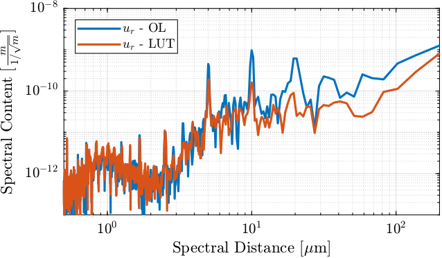
Figure 18: Effect of the LUT on the spectral content of the positioning errors
Let’s now look at it in a cumulative way.
CPS_ol_ur = flip(-cumtrapz(flip(f), flip(S_ol_ur)));
CPS_ol_uh = flip(-cumtrapz(flip(f), flip(S_ol_uh)));
CPS_ol_d  = flip(-cumtrapz(flip(f), flip(S_ol_d)));

CPS_lut_ur = flip(-cumtrapz(flip(f), flip(S_lut_ur)));
CPS_lut_uh = flip(-cumtrapz(flip(f), flip(S_lut_uh)));
CPS_lut_d  = flip(-cumtrapz(flip(f), flip(S_lut_d)));
%% Cumulative Spectrum
figure;
hold on;
plot(1e6./f, sqrt(CPS_ol_ur) , 'DisplayName', '$u_r$ - OL');
plot(1e6./f, sqrt(CPS_lut_ur), 'DisplayName', '$u_r$ - LUT');
hold off;
set(gca, 'xscale', 'log'); set(gca, 'yscale', 'log');
xlabel('Spectral Distance [$\mu m$]'); ylabel('Cumulative Spectrum [$m$]')
xlim([1, 500]); ylim([1e-9, 1e-5]);
legend('location', 'northwest');
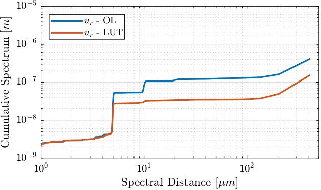
Figure 19: Cumulative Spectrum with and without the LUT
2.6. Period of errors
The positioning errors of the fast jacks have different origins with different spatial periods:
- \(1mm\) due to non-perfect planetary roller screw system
- \(20\mu m\), \(10\mu m\) and \(5\mu m\) periods due non-perfect magnetic poles of the stepper motor.
In this section, we wish to see which of these errors are repeatable from one scan to the other. This could help to determine which errors should be included in the LUT.
2.6.0.1. Load Test Data
A scan in mode A is performed at constant Fast Jack velocity.
fj_vel = 0.125e-3; % Fast Jack Velocity [m/s]
2.6.0.2. FIR Filters
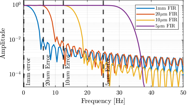
Figure 20: Amplitude response of FIR filters to only keep certain errors
2.6.0.3. Filtered Data
Now the same data is filtered with each filter.
The filtered data are shown in Figure 21.
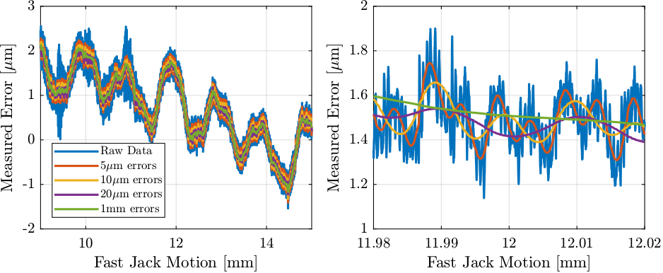
Figure 21: Fast Jack measured error and filtered data
2.6.0.4. Discussion
3. LUT creation from experimental data
In this section, the full process from measurement, filtering of data to generation of the LUT is detailed.
The computation is performed with Matlab.
3.1. Load Data
A Bragg scan is performed using thtraj and data are acquired using the fast_DAQ.
%% Load Raw Data
load("scan_10_70_lut_1.mat")
Measured data are:
bragg: Bragg angle in degdz: distance between crystals in nmdry,drx: orientation errors between crystals in nradfjur,fjuh,fjd: generated steps by the IcePAP in tens of nm
All are sampled at 10kHz with no filtering.
First, convert all the data to SI units (rad, and m).
%% Convert Data to Standard Units
% Bragg Angle [rad]
bragg = pi/180*bragg;
% Rx rotation of 1st crystal w.r.t. 2nd crystal [rad]
drx   = 1e-9*drx;
% Ry rotation of 1st crystal w.r.t. 2nd crystal [rad]
dry   = 1e-9*dry;
% Z distance between crystals [m]
dz    = 1e-9*dz;
% Z error between second crystal and first crystal [m]
ddz   = 10.5e-3./(2*cos(bragg)) - dz;
% Steps for Ur motor [m]
fjur  = 1e-8*fjur;
% Steps for Uh motor [m]
fjuh  = 1e-8*fjuh;
% Steps for D motor [m]
fjd   = 1e-8*fjd;
3.2. IcePAP generated Steps
Here is how the steps of the IcePAP (fjsur, fjsuh and fjsd) are computed in mode A:
There is a first offset \(\text{fjs}_0\) that is initialized once, and a second offset which is a function of fjsry and fjsrx.
Let’s compute the offset which is a function of fjsry and fjsrx:
fjsry = 0.53171e-3; % [rad]
fjsrx = 0.144e-3;   % [rad]

J_a_111 = [1,  0.14, -0.0675
           1,  0.14,  0.1525
           1, -0.14,  0.0425];

fjs_offset = J_a_111*[0; fjsry; fjsrx]; % ur,uh,d offsets [m]
| 6.4719e-05 |
| 9.6399e-05 |
| -6.8319e-05 |
Let’s now compute \(\text{fjs}_0\) using first second of data where there is no movement and bragg axis is fixed at \(\theta_0\):
\begin{equation} \text{fjs}_0 = \begin{bmatrix} \text{fjsur} \\ \text{fjsuh} \\ \text{fjsd} \end{bmatrix} (\theta_0) + \frac{10.5 \cdot 10^{-3}}{2 \cos (\theta_0)} - \bm{J}_{a,111} \cdot \begin{bmatrix} 0 \\ \text{fjsry} \\ \text{fjsrx} \end{bmatrix} \end{equation}FJ0 = ... mean([fjur(time < 1), fjuh(time < 1), fjd(time < 1)])' ... + ones(3,1)*10.5e-3./(2*cos(mean(bragg(time < 1)))) ... - fjs_offset; % [m]
| 0.030427 |
| 0.030427 |
| 0.030427 |
Values are very close for all three axis. Therefore we take the mean of the three values for \(\text{fjs}_0\).
FJ0 = mean(FJ0);
This approximately corresponds to the distance between the crystals for a Bragg angle of 80 degrees:
10.5e-3/(2*cos(80*pi/180))
0.030234
The measured IcePAP steps are compared with the theoretical formulas in Figure 22.
If we were to zoom a lot, we would see a small delay between the estimation and the steps sent by the IcePAP. This is due to the fact that the estimation is performed based on the measured Bragg angle while the IcePAP steps are based on the “requested” Bragg angle. As will be shown in the next section, there is a small delay between the requested and obtained bragg angle which explains this delay.
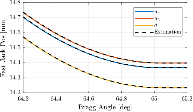
Figure 22: Measured IcePAP Steps and estimation from theoretical formula
3.3. Bragg and Fast Jack Velocities
In order to estimate velocities from measured positions, a filter is used which approximate a pure derivative filter.
%% Filter to compute velocities
G_diff = (s/2/pi/10)/(1 + s/2/pi/10);
% Make sure the gain w = 2pi is equal to 2pi
G_diff = 2*pi*G_diff/(abs(evalfr(G_diff, 1j*2*pi)));
Only the high frequency amplitude is reduced to not amplified the measurement noise (Figure 23).
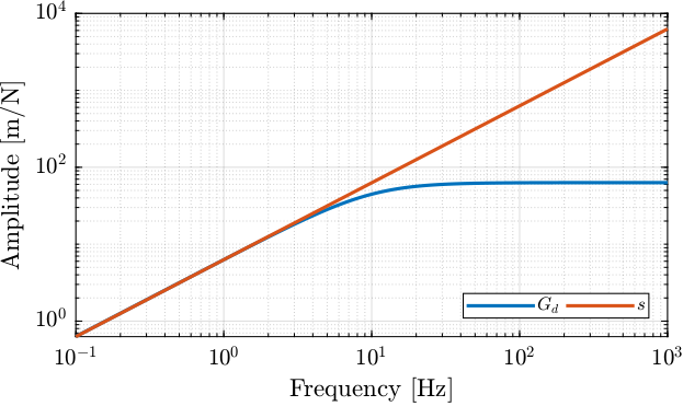
Figure 23: Magnitude of filter used to approximate the derivative
Using the filter, the Bragg velocity is estimated (Figure 24).
%% Bragg Velocity
bragg_vel = lsim(G_diff, bragg, time);
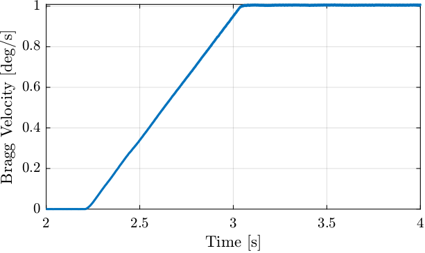
Figure 24: Estimated Bragg Velocity curing acceleration phase
Now, the Fast Jack velocity is estimated (Figure 25).
%% Fast Jack Velocity
fjur_vel = lsim(G_diff, fjur, time);
fjuh_vel = lsim(G_diff, fjuh, time);
fjd_vel  = lsim(G_diff, fjd , time);
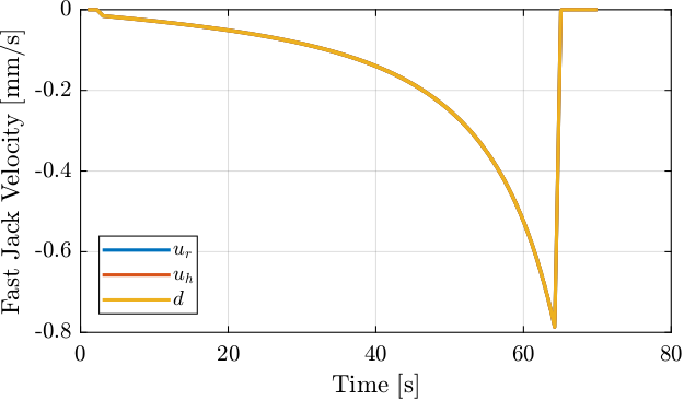
Figure 25: Estimated velocity of fast jacks
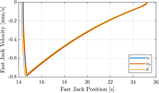
Figure 26: Fast Jack Velocity as a function of its position
3.4. Bragg Angle Errors / Delays
From the measured fjur steps generated by the IcePAP, we can estimate the steps generated corresponding to the Bragg angle.
%% Estimated Bragg angle requested by IcePAP
bragg_icepap = acos(10.5e-3./(2*(FJ0 + fjs_offset(1) - fjur)));
The generated steps by the IcePAP and the measured angle are compared in Figure 27. There is clearly a lag of the Bragg angle compared to the generated IcePAP steps.
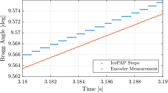
Figure 27: Estimated generated steps by the IcePAP and measured Bragg angle
If we plot the error between the measured and the requested bragg angle as a function of the bragg velocity (Figure 28), we can see an almost linear relationship.
This corresponds to a “time lag” of approximately:
2.4 ms
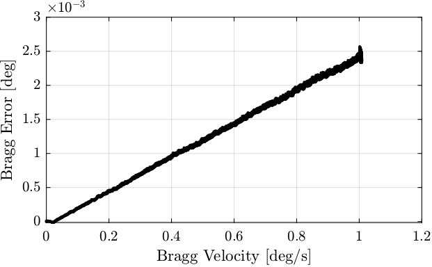
Figure 28: Bragg Error as a function fo the Bragg Velocity
There is a “lag” between the Bragg steps sent by the IcePAP and the measured angle by the encoders. This is probably due to the single integrator in the “Aerotech” controller. Indeed, two integrators are required to have no tracking error during ramp reference signals.
3.5. Errors in the Frame of the Crystals
The dz, dry and drx measured relative motion of the crystals are defined as follows:
- An increase of
dzmeans the crystals are moving away from each other - An positive
drymeans the second crystals has positive rotation aroundy - An positive
drxmeans the second crystals has positive rotation aroundx
The error in crystals’ distance ddz is defined as:
Therefore, a positive ddz means that the second crystal is too high (fast jacks have to move down).
The errors measured in the frame of the crystals are shown in Figure 29.
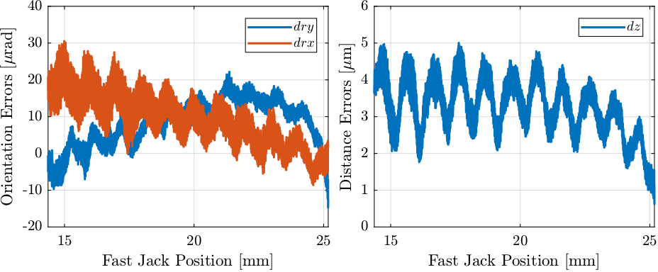
Figure 29: Measured errors in the frame of the crystals as a function of the fast jack position
3.6. Errors in the Frame of the Fast Jacks
From ddz,dry,drx, the motion errors of the jast-jacks (fjur_e, fjuh_e and jfd_e) as measured by the interferometers are computed.
%% Actuator Jacobian
J_a_111 = [1,  0.14, -0.0675
           1,  0.14,  0.1525
           1, -0.14,  0.0425];

%% Computation of the position of the FJ as measured by the interferometers
error = J_a_111 * [ddz, dry, drx]';

fjur_e = error(1,:)'; % [m]
fjuh_e = error(2,:)'; % [m]
fjd_e  = error(3,:)'; % [m]
The result is shown in Figure 30.
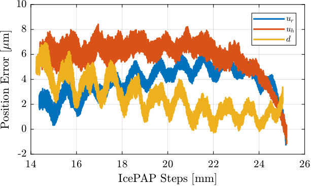
Figure 30: Position error of the Fast jacks
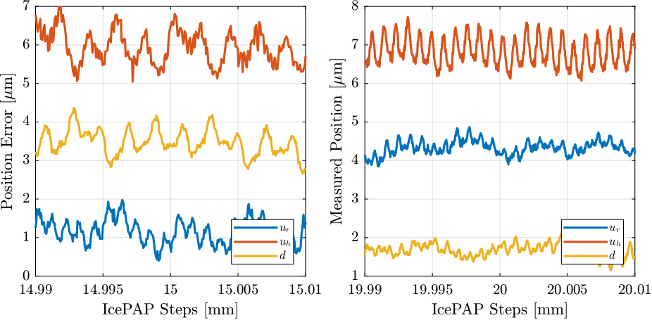
Figure 31: Position error of the Fast jacks - Zoom near two positions
3.7. Analysis of the obtained error
The measured position of the fast jacks are displayed as a function of the IcePAP steps (Figure 32).
From Figure 32, it seems the position as a function of the IcePAP steps is not a bijection function. Therefore, a measured position can corresponds to several IcePAP Steps. This is very problematic for building a LUT that will be used to compensated the measured errors.
Also, it seems that the (spatial) period of the error depends on the actual position of the Fast Jack (and therefore of its velocity). If we compute the equivalent temporal period, we find a frequency of around 370 Hz.
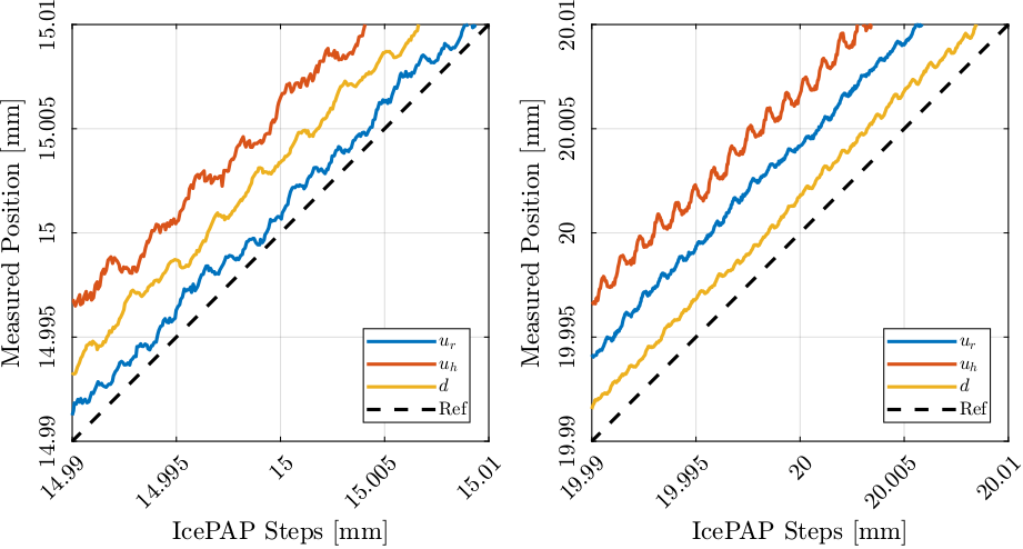
Figure 32: Measured Fast Jack position as a function of the IcePAP steps
In order to better investigate what is going on, a spectrogram is computed (Figure 33).
We clearly observe:
- Some rather constant vibrations with a frequency at around 363Hz and 374Hz.
This corresponds to the clear periods in Figure 32.
These are due to the
mcoilstepper motor (magnetic period). - Several frequencies which are increasing with time. These corresponds to (spatial) periodic errors of the stepper motor. The frequency of these errors are increasing because the velocity of the fast jack is also increasing with time (see Figure 25). The black dashed line in Figure 33 shows the frequency of errors with a period of \(5\,\mu m\). We can also see lower frequencies corresponding to periods of \(10\,\mu m\) and \(20\,\mu m\) and lots of higher frequencies with are also exciting resonances of the system (second crystal) at around 200Hz
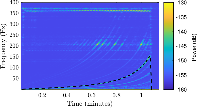
Figure 33: Spectrogram of the \(u_h\) errors. The black dashed line corresponds to an error with a period of \(5\,\mu m\)
As we would like to only measure the repeatable mechanical errors of the fast jacks and not the vibrations of natural frequencies of the system, we have to filter the data.
3.8. Filtering of Data
As seen in Figure 33, the errors we wish to calibrate are below 160Hz while the vibrations we wish to ignore are above 200Hz. We have to use a low pass filter that does not affects frequencies below 160Hz while having good rejection above 200Hz.
The filter used for current LUT is a moving average filter with a length of 100:
%% Moving Average Filter
B_mov_avg = 1/101*ones(101,1); % FIR Filter coeficients
We may also try a second order low pass filter:
%% 2nd order Low Pass Filter
G_lpf = 1/(1 + 2*s/(2*pi*80) + s^2/(2*pi*80)^2);
And a FIR filter with linear phase:
%% FIR with Linear Phase
Fs = 1e4; % Sampling Frequency [Hz]
B_fir = firls(1000, ... % Filter's order
              [0 140/(Fs/2) 180/(Fs/2) 1], ... % Frequencies [Hz]
              [1 1          0          0]); % Wanted Magnitudes
Filters’ responses are computed and compared in the Bode plot of Figure 34.
%% Computation of filters' responses
[h_mov_avg, f] = freqz(B_mov_avg, 1, 10000, Fs);
[h_fir,     ~] = freqz(B_fir,     1, 10000, Fs);
h_lpf          = squeeze(freqresp(G_lpf,  f, 'Hz'));
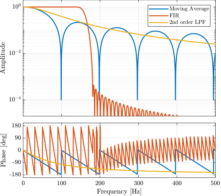
Figure 34: Bode plot of filters that could be used before making the LUT
Clearly, the currently used moving average filter is filtering too much below 160Hz and too little above 200Hz. The FIR filter seems more suited for this case.
Let’s now compare the filtered data.
fjur_e_cur = filter(B_mov_avg, 1, fjur_e);
fjur_e_fir = filter(B_fir,     1, fjur_e);
fjur_e_lpf = lsim(G_lpf, fjur_e, time);
As the FIR filter introduce some delays, we can identify this relay and shift the filtered data:
%% Compensate the FIR delay
delay = mean(grpdelay(B_fir));
500
fjur_e_fir(1:end-delay) = fjur_e_fir(delay+1:end);
The same is done for the moving average filter
%% Compensate the Moving average delay
delay = mean(grpdelay(B_mov_avg));
fjur_e_cur(1:end-delay) = fjur_e_cur(delay+1:end);
The raw and filtered motion errors are displayed in Figure 35.
It is shown that while the moving average average filter is working relatively well for low speeds (at around 20mm) it is not for high speeds (near 15mm). This is because the frequency of the error is above 100Hz and the moving average is flipping the sign of the filtered data.
The IIR low pass filter has some phase issues.
Finally the FIR filter is perfectly in phase while showing good attenuation of the disturbances.
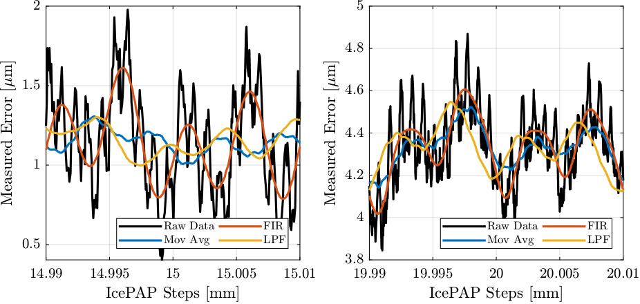
Figure 35: Raw measured error and filtered data
If we now look at the measured position as a function of the IcePAP steps (Figure 36), we can see that we obtain a monotonous function for the FIR filtered data which is great to make the LUT.
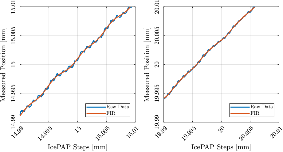
Figure 36: Raw measured motion and filtered motion as a function of the IcePAP Steps
If we subtract the raw data with the FIR filtered data, we obtain the remaining motion shown in Figure 37 that only contains the high frequency motion not filtered.
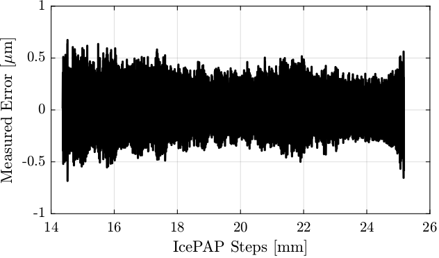
Figure 37: Remaining motion error after removing the filtered part
3.9. LUT creation
The procedure used to make the Lookup Table is schematically represented in Figure 38.
For each IcePAP step separated by a constant value (typically \(1\,\mu m\)) a point of the LUT is computed:
- Points where the measured position is close to the wanted ideal position (i.e. the current IcePAP step) are found
- The corresponding IcePAP step at which the Fast Jack is at the wanted position is stored in the LUT
Therefore the LUT gives the IcePAP step for which the fast jack is at the wanted position as measured by the metrology, which is what we want.
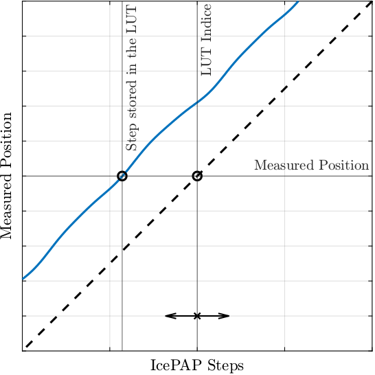
Figure 38: Schematic of the principle used to make the Lookup Table
Let’s first initialize the LUT which is table with 4 columns and 26001 rows. The columns are:
- IcePAP Step indices from 0 to 26mm with a step of \(1\,\mu m\) (thus the 26001 rows)
- IcePAP step for
fjurat which point the fast jack is at the wanted position - Same for
fjuh - Same for
fjd
All the units of the LUT are in mm. We will work in meters and convert to mm at the end.
Let’s initialize the Lookup table:
%% Initialization of the LUT
lut = [0:1e-6:26e-3]'*ones(1,4);
And verify that it has the wanted size:
size(lut)
ans =
       26001           4
The measured Fast Jack position are filtered using the FIR filter:
%% FIR Filter
Fs = 1e4; % Sampling Frequency [Hz]
fir_order = 1000; % Filter's order
delay = fir_order/2; % Delay induced by the filter
B_fir = firls(fir_order, ... % Filter's order
              [0 140/(Fs/2) 180/(Fs/2) 1], ... % Frequencies [Hz]
              [1 1          0          0]); % Wanted Magnitudes

%% Filtering all measured Fast Jack Position using the FIR filter
fjur_e_filt = filter(B_fir, 1, fjur_e);
fjuh_e_filt = filter(B_fir, 1, fjuh_e);
fjd_e_filt  = filter(B_fir, 1, fjd_e);

%% Compensation of the delay introduced by the FIR filter
fjur_e_filt(1:end-delay) = fjur_e_filt(delay+1:end);
fjuh_e_filt(1:end-delay) = fjuh_e_filt(delay+1:end);
fjd_e_filt( 1:end-delay) = fjd_e_filt( delay+1:end);
The indices where the LUT will be populated are initialized.
%% Vector of Fast Jack positions [unit of lut_inc]
fjur_pos = floor(min(1e6*fjur)):floor(max(1e6*fjur));
fjuh_pos = floor(min(1e6*fjuh)):floor(max(1e6*fjuh));
fjd_pos  = floor(min(1e6*fjd )):floor(max(1e6*fjd ));
And the LUT is computed and shown in Figure 39.
%% Build the LUT
for i = fjur_pos
    % Find indices where measured motion is close to the wanted one
    indices = fjur + fjur_e_filt > lut(i,1) - 500e-9 & ...
              fjur + fjur_e_filt < lut(i,1) + 500e-9;
    % Poputate the LUT with the mean of the IcePAP steps
    lut(i,2) = mean(fjur(indices));
end

for i = fjuh_pos
    % Find indices where measuhed motion is close to the wanted one
    indices = fjuh + fjuh_e_filt > lut(i,1) - 500e-9 & ...
              fjuh + fjuh_e_filt < lut(i,1) + 500e-9;
    % Poputate the LUT with the mean of the IcePAP steps
    lut(i,3) = mean(fjuh(indices));
end

for i = fjd_pos
    % Poputate the LUT with the mean of the IcePAP steps
    indices = fjd + fjd_e_filt > lut(i,1) - 500e-9 & ...
              fjd + fjd_e_filt < lut(i,1) + 500e-9;
    % Poputate the LUT
    lut(i,4) = mean(fjd(indices));
end
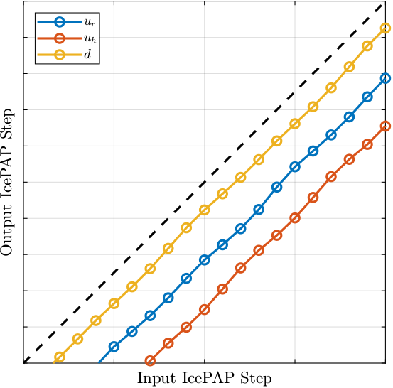
Figure 39: Lookup Table correction
3.10. Cubic Interpolation of the LUT
Once the LUT is built and loaded to the IcePAP, generated steps are taking the step values in the LUT and cubic spline interpolation is performed.
%% Estimation of the IcePAP output steps after interpolation
fjur_out_steps = spline(lut(:,1), lut(:,2), fjur);
The LUT data points as well as the spline interpolation values and the ideal values are compared in Figure 40. It is shown that the spline interpolation seems to be quite accurate.
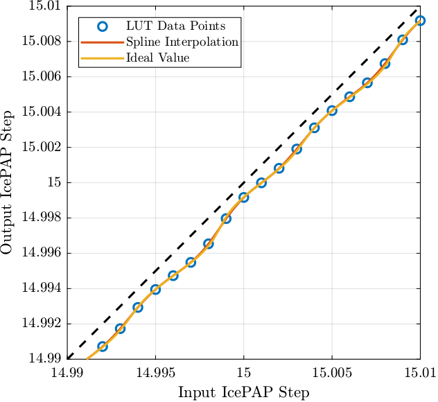
Figure 40: Output IcePAP Steps avec spline interpolation compared with the ideal steps
The difference between the perfect step generation and the step generated after spline interpolation is shown in Figure 41. The remaining position error is in the order of 100nm peak to peak which is acceptable here.
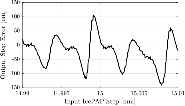
Figure 41: Errors on the computed IcePAP output steps after LUT generation and spline interpolation
In order to limit the errors due to spline interpolation, more points in the LUT should be included (ideally one point every 100nm). This only makes the computation of the LUT a little bit longer.
4. Position Repeatability
In this section, the repeatability of the Fast Jacks over time is studied.
The goal is to determine:
- How good the positioning accuracy can be when using the Lookup Table to correct the non-repeatability of the fast jack motion (i.e. mode B)?
- During how long the lookup table are remaining valid?
- Which errors are repeatable and which are not?
The trajectories to test the repeatability is the following:
tdh.lut_constant_fj_vel(15, 22, pts_per_mm=1000, use_lut=False)
The Fast Jack are scanned at constant velocity from 22mm to 15mm in mode A (no LUT). The velocity is set to 0.125mm/s.
4.1. Repeatability over several minutes
10 scans are done one after the other in mode A.
%% Filenames for the measurements
data_files_min = {
    "lut_const_fj_vel_14012022_1517.dat",
    "lut_const_fj_vel_14012022_1519.dat",
    "lut_const_fj_vel_14012022_1521.dat",
    "lut_const_fj_vel_14012022_1523.dat",
    "lut_const_fj_vel_14012022_1525.dat",
    "lut_const_fj_vel_14012022_1527.dat",
    "lut_const_fj_vel_14012022_1528.dat",
    "lut_const_fj_vel_14012022_1530.dat",
    "lut_const_fj_vel_14012022_1532.dat",
    "lut_const_fj_vel_14012022_1534.dat"
};
The data are filtered such that most of the disturbances and noise are filtered out.
There is only the motion errors induced by the fast jack left in the data.
The measured position errors of fjur are shown in Figure 42 for the 10 scans.
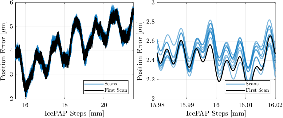
Figure 42: Repeatability of fjur over several minutes
The non-repeatable part (measured motion of scan i minus the measured motion of the first scan) is shown in Figure 43. Visually, we see that we cannot expect the positioning errors to be less than several hundreds of nanometers in mode B.
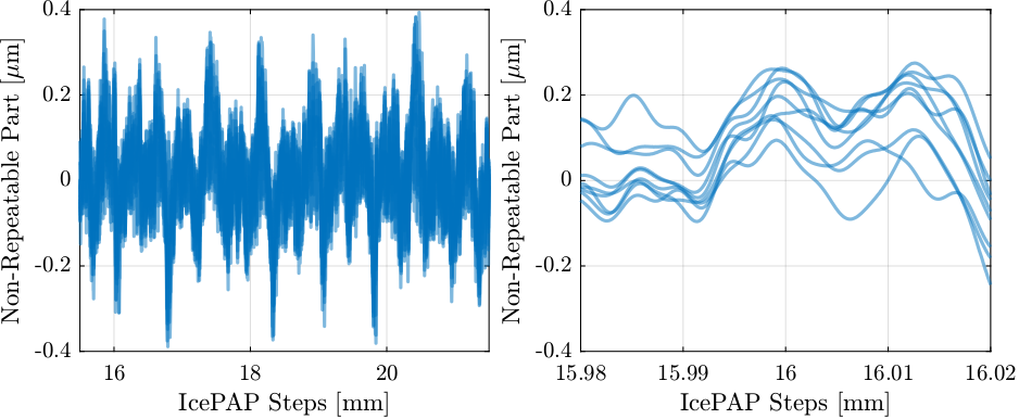
Figure 43: Non Repeatable part over several minutes
The RMS value of the non repeatable part is computed for each scan and summarized in Table 1. It is visually shown in Figure 44.
Clearly, the error is getting worse as more scan are performed and/or as elapse time is longer.
| Elapse Time [m] | fjur [nm] |
fjuh [nm] |
fjd [nm] |
|---|---|---|---|
| 2.0 | 47.9 | 32.4 | 38.1 |
| 4.0 | 62.5 | 42.0 | 54.1 |
| 6.0 | 74.7 | 50.4 | 66.0 |
| 8.0 | 85.8 | 53.7 | 81.3 |
| 10.0 | 95.0 | 59.9 | 90.4 |
| 11.0 | 104.6 | 65.3 | 98.0 |
| 13.0 | 115.7 | 68.6 | 105.6 |
| 15.0 | 126.8 | 68.4 | 112.6 |
| 17.0 | 138.4 | 70.8 | 123.2 |
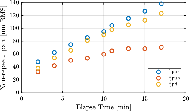
Figure 44: Remaining motion as a function of the elapse time / number of iteration
4.2. Repeatability over several days
The same scan is done with approximately 8 hours of time interval over three days.
%% Filenames for the measurements
data_files_day = {
    "lut_const_fj_vel_14012022_1824.dat",
    "lut_const_fj_vel_15012022_0234.dat",
    "lut_const_fj_vel_15012022_1043.dat",
    "lut_const_fj_vel_15012022_1852.dat",
    "lut_const_fj_vel_16012022_0302.dat",
    "lut_const_fj_vel_16012022_1111.dat",
    "lut_const_fj_vel_16012022_1920.dat"
};
The measured position errors of fjur during all the scans are shown in Figure 45.
Clearly, the repeatability is worse than when the scans where only spaced by few minutes (Figure 42).
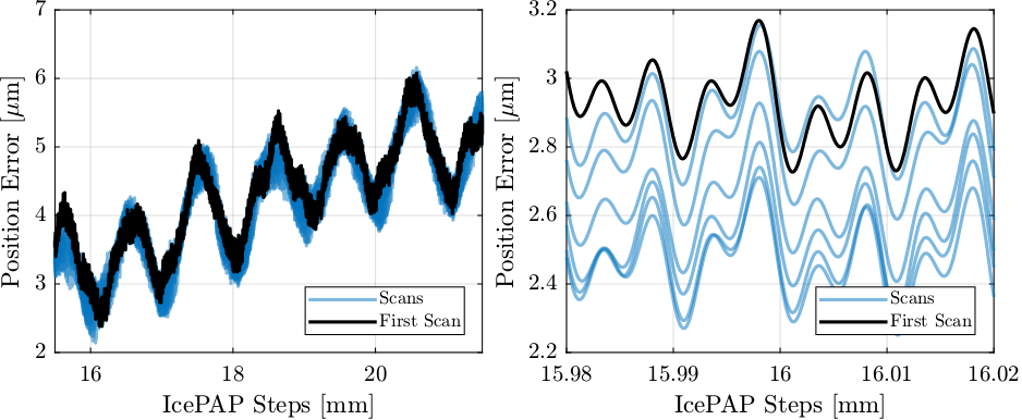
Figure 45: Repeatability of fjur over several hours
The non-repeatable part is computed, summarized in Table 2 and visually shown in Figure 46.
| Elapse Time [days] | fjur [nm] |
fjuh [nm] |
fjd [nm] |
|---|---|---|---|
| 0.3 | 102.9 | 65.4 | 76.0 |
| 0.7 | 147.3 | 75.1 | 91.5 |
| 1.0 | 188.8 | 86.9 | 106.2 |
| 1.4 | 220.8 | 97.2 | 107.2 |
| 1.7 | 244.2 | 106.6 | 104.3 |
| 2.0 | 252.7 | 117.6 | 106.1 |
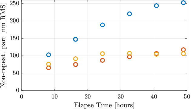
Figure 46: RMS value of the non-repeatable part for scans spaced by 8 hours
4.3. Which error is repeatable and which is not?
In the previous section, it was shown that the non-repeatable part of the fast jack motion is in the order of several hundreds of nano-meters.
In this section, we wish to see if this non-repeatable error is due to:
- Thermal drifts?
- non-repeatability of the ball-screw mechanism (1mm error period)
- non-repeatability of the \(20\mu m/10\mu m/5\mu m\) period errors
To do so, a spectral analysis of the non-repeatable part is performed.
First, we look at the errors with small spatial periods in Figure 47. It is clear that:
- errors with periods of \(5\mu m\) and \(20\mu m\) are very repeatable over several days
- errors with periods of \(10\mu m\) are well repeatable over several minutes but less over not hours/days (Figure 47, right)
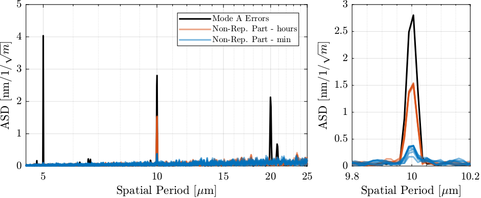
Figure 47: ASD of the non-repeatable motion part for scans spaced by several minutes and by several hours
The errors related to large spatial periods are shown in Figure 48. Two errors can be observed:
- 1mm error period with good repeatability. This repeatability degrades with time / number of scans. Still well after several days.
- 0.37mm error period. Well repeatable for the first scan after 2 minutes. Degrades quickly.
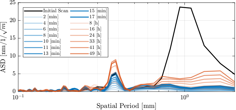
Figure 48: (Spatial) Spectral Density of the non-repeatability with large spatial periods
The repeatability is very good for the \(5\,\mu m\) and \(20\,\mu m\) period errors (Figure 47), a little bit less for the \(10\,\mu m\) error period (Figure 47, right). What can be the physical cause of that?
The non-repeatability with large spatial periods are degrading over time (Figure 48). They are however more easily compensated with the feedback control (mode C).
The cause of the error with a period of 0.37mm is still unknown.
4.4. Estimation of the errors in mode B
In this section, the expected errors in mode B are estimated.
In order to do so the LUT for the initial scan is computed and then applied to the following scans.
%% Filenames for the measurements
data_files_min = {
    "lut_const_fj_vel_14012022_1517.dat",
    "lut_const_fj_vel_14012022_1519.dat",
    "lut_const_fj_vel_14012022_1521.dat",
    "lut_const_fj_vel_14012022_1523.dat",
    "lut_const_fj_vel_14012022_1525.dat",
    "lut_const_fj_vel_14012022_1527.dat",
    "lut_const_fj_vel_14012022_1528.dat",
    "lut_const_fj_vel_14012022_1530.dat",
    "lut_const_fj_vel_14012022_1532.dat",
    "lut_const_fj_vel_14012022_1534.dat"
};
Let’s first do this analysis for the first two scans and for the fjur fast jack.
The measured motion errors are shown in Figure 49 (left) and the difference between the measured motion in Figure 49 (right).
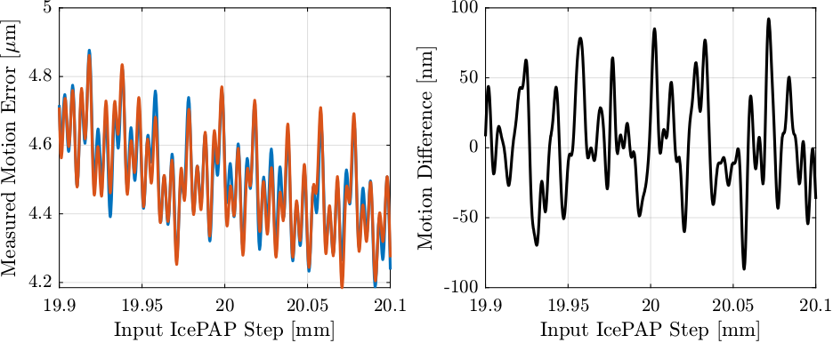
Figure 49: Measured motion error for fjur during both scans (left) and difference in the measured motion (right)
Let’s now compare the LUT that are computed from both scans (Figure 50). The two LUT corrections are differing by about 50 nm RMS.
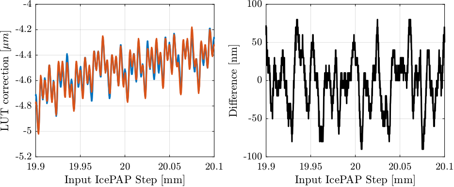
Figure 50: Generated fjur LUT for both scans (left) and differences between the LUT (right)
Let’s now estimate the motion error in mode B is the LUT computed with the first scan were used.
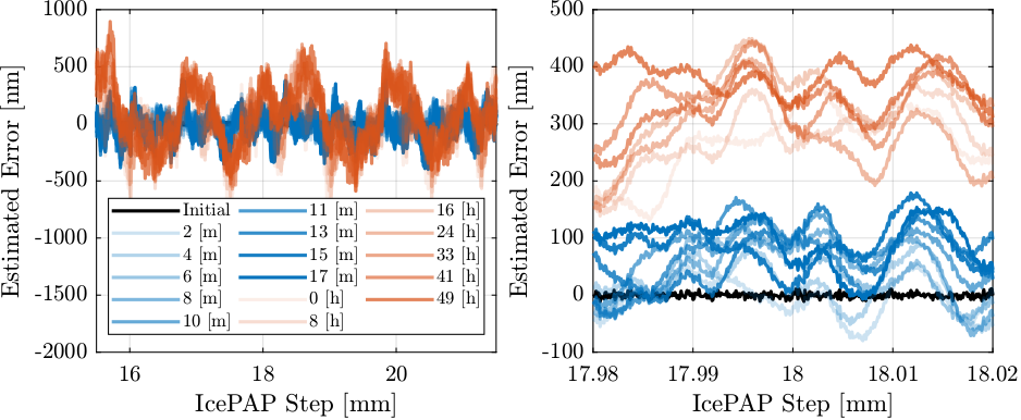
Figure 51: Estimated error on fjur using LUT made based on the first scan
The RMS value of the remaining error in mode B for fjur are computed and summarized in Table 3.
The error is increasing over first half hour and seems to stabilize after several hours.
| Elapse Time [h] | fjur [nm RMS] |
|---|---|
| 0.0 | 48.1 |
| 0.1 | 62.9 |
| 0.1 | 75.1 |
| 0.1 | 86.1 |
| 0.2 | 95.4 |
| 0.2 | 105.0 |
| 0.2 | 115.7 |
| 0.2 | 126.8 |
| 0.3 | 138.3 |
| 8.2 | 247.4 |
| 16.3 | 240.9 |
| 24.5 | 234.2 |
| 32.6 | 232.9 |
| 40.8 | 249.0 |
| 48.9 | 270.7 |
The (spatial) spectral density of the estimated errors in mode B are computed and shown in Figure 52 for short spatial periods and in Figure 53 for large spatial errors.
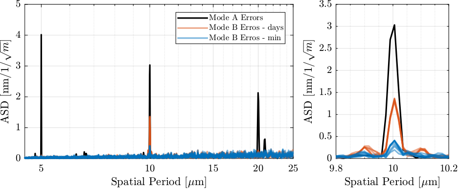
Figure 52: Estimated spectral density of the fjur errors in mode B for several scans. Focus on short spatial periods.
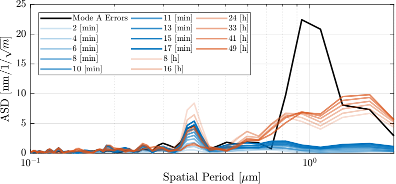
Figure 53: Estimated spectral density of the fjur errors in mode B for several scans. Focus on large spatial periods.
Using the LUT, most of the errors can be compensated. This includes the errors of the stepper motor (with periods of \(5\,\mu m\), \(10\,\mu m\) and \(20\,\mu m\)) and the errors of the ball-screw mechanism (periods of \(1\,mm\)).
The “quality” of the LUT is degrading over time, especially for periods of \(10\,\mu m\) and \(1\,mm\). While the errors with a period of \(1\,mm\) are not an issue as they will be easily compensated using feedback control, errors with a period of \(10\,\mu m\) could be more problematic.
4.5. Conclusion
Repeatability of the Fast Jack motion has been studied.
Even though the repeatability degrades over time, the main errors with a period of \(5\,\mu m\) are well repeatable over many scans and time spans of several days. The degradation of the repeatability is mostly problematic of the errors with a period of \(10\,\mu m\).
It was shown that the use of a Lookup Table can eliminate most of the repeatable errors. The remaining motion error on each fast jack is expected to be in the order of \(100\,nm \text{RMS}\) (see Figure 51).
5. LUT Software Implementation
5.1. Matlab implementation
5.1.1. LUT Creation
A scan in mode A is performed using the thtraj motor.
The scan is performed from 10 to 70 degrees.
%% Extract measurement Data make from BLISS
data_A = extractDatData(sprintf("%s/21Nov/blc13420/id21/LUT_Matlab/lut_matlab_22122021_1610.dat", data_directory), ...
                     {"bragg", "dz", "dry", "drx", "fjur", "fjuh", "fjd"}, ...
                     [pi/180, 1e-9, 1e-9, 1e-9, 1e-8, 1e-8, 1e-8]);
A LUT is generated from this Data.
%% Generate LUT
data_lut = createLUT(data_A, "./matlab/lut/lut_matlab_22122021_1610_10_70_table.dat");
The generated LUT is shown in Figure 54.
Figure 54: Generated LUT
5.1.2. Compare Mode A and Mode B
The LUT is loaded into the IcePAP and a new scan in mode B is performed over the same stroke.
%% Load mode B scan data
data_B = extractDatData(sprintf("%s/21Nov/blc13420/id21/LUT_Matlab/lut_matlab_result_22122021_1616.dat", data_directory), ...
                     {"bragg", "dz", "dry", "drx", "fjur", "fjuh", "fjd"}, ...
                     [pi/180, 1e-9, 1e-9, 1e-9, 1e-8, 1e-8, 1e-8]);
The raw (unfiltered, 10kHz) measured motion for fjur, fjuh and fjd are displayed in Figure 55.
Figure 55: Comparison of the Raw measurement of fast jack motion errors for mode A and mode B
As the raw measured data is quite noisy and affected by disturbances, the data is filtered to obtain the motion errors of the fast jack. The filtered measured errors are shown in Figure 56.
Figure 56: Comparison of the Raw measurement of fast jack motion errors for mode A and mode B
5.1.3. Analysis of the remaining errors
Let’s now analyze the remaining errors.
The spectral content of the errors are shown in Figure 57. The following can be observed:
- errors with periods of \(5\,\mu m\), \(10\,\mu m\) and \(20\,\mu m\) are reduced
- errors with period of 0.37mm and 1mm are almost totally reduced
- additional motion are added in mode B with periods from \(15\,\mu m\) to \(25\,\mu m\)
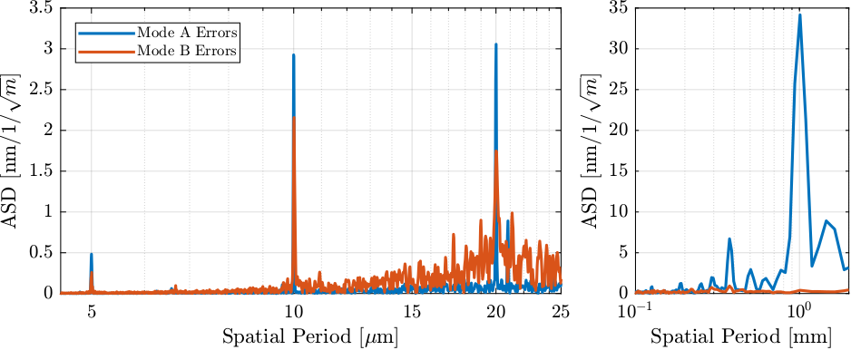
Figure 57: Spectral density of the fjur measured errors in mode A and mode B
Even though the errors in mode B are well reduced as compared to mode A, the LUT is not working as well as expected from Section 4.4.
This can be due to several factors:
- limited number of points taken in the LUT (original 1 point every \(\mu m\)) which leads to errors when interpolating the LUT
- limited number of points taken in the mode B trajectory leading to interpolation errors
Further tests will be performed with in more ideal conditions:
- better trajectory used to build the LUT
- more points in the LUT as well as in the trajectory
5.2. Python implementation
5.2.1. Load Data
A scan in mode A is performed and loaded.
data = np.loadtxt("/home/thomas/mnt/data_id21/21Nov/blc13420/id21/LUT_constant_fj_vel/lut_const_fj_vel_17012022_1749.dat")
Useful data are extracted and converted to SI units.
bragg = np.pi/180*data[:,0] # Bragg Angle [rad]
dz = 1e-9*data[:,1] # Distance between crystals [m]
dry = 1e-9*data[:,2] # dry [rad]
drx = 1e-9*data[:,3] # drx [rad]
fjur = 1e-8*data[:,4] # ur Fast Jack Step in [m]
fjuh = 1e-8*data[:,5] # uh Fast Jack Step in [m]
fjd = 1e-8*data[:,6] # d Fast Jack Step in [m]
time = 1e-4*np.arange(0, np.size(bragg), 1) # Time vector [s]
ddz = 10.5e-3/(2*np.cos(bragg)) - dz; # Z error between the two crystals [m]
The Bragg angle as a function of time is shown in Figure 58 and the fast jack displacements are shown in Figure 59.
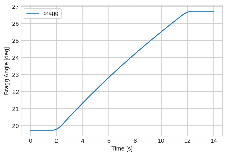
Figure 58: Bragg angle during the mode A scan

Figure 59: Fast Jack motion during the mode A scan
5.2.2. Convert Data in the frame of the fast jack
The measured motion of the crystals using the interferometers are converted to the motion of the three jacks using the Jacobian matrix.
# Actuator Jacobian
J_a_111 = np.array([[1,  0.14, -0.0675], [1,  0.14,  0.1525], [1, -0.14,  0.0425]])

# Computation of the position of the FJ as measured by the interferometers
error = J_a_111 @ [ddz, dry, drx]

fjur_e = error[0,:] # [m]
fjuh_e = error[1,:] # [m]
fjd_e  = error[2,:] # [m]
The obtained motion error of the fast jack as a function of time are shown in Figure 60.
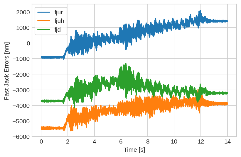
Figure 60: Measured fast jack motion errors as a function of time
5.2.3. Filter Data
In order to get rid of external disturbances and noise, the measured fast jack displacement errors are low pass filtered.
The filter parameters are defined below.
# Generate Low pass FIR Filter
sample_rate = 10000.0 # Sample Rate [Hz]
nyq_rate = sample_rate / 2.0 # Nyquist Rate [Hz]

cutoff_hz = 27 # The cutoff frequency of the filter [Hz]

# Window with specific ripple [dB] and width [Nyquist Fraction]
N, beta = kaiserord(60, 4/nyq_rate)

# Delay expressed in number of sample
N_delay = int((N-1)/2)

# Delay expressed in seconds
delay = N_delay / sample_rate
The filter is generated using the following command:
# Fitler generation
taps = firwin(N, cutoff_hz/nyq_rate, window=('kaiser', beta))
This filter will introduce a constant delay that is a function of its length:
print("Length of the filter is %i\nDelay is %i samples (i.e. %.3f seconds)" % (N, N_delay, delay))
Length of the filter is 9065
Delay is 4532 samples (i.e. 0.453 seconds)
The measured data is then filtered using the lfilter command.
The obtained raw and filtered data are displayed in Figure 61.
# Filtering of data, compensation of the delay introduced by the FIR filter
fjur_e_filt = lfilter(taps, 1.0, fjur_e)[N:]
fjuh_e_filt = lfilter(taps, 1.0, fjuh_e)[N:]
fjd_e_filt = lfilter(taps, 1.0, fjd_e)[N:]
time_filt = time[N_delay+1:-N_delay]
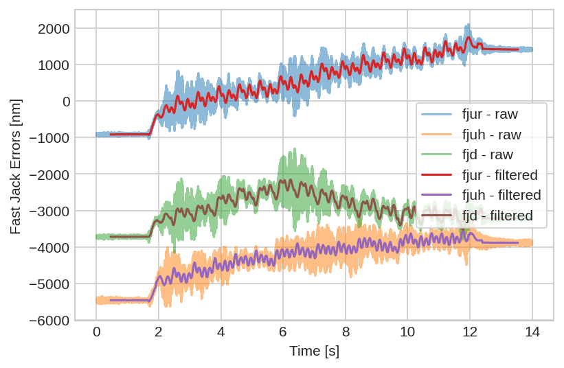
Figure 61: Raw and filtered measured errors of the fast jack motion
The measured fast jack motion (filtered) as a function of the IcePAP steps (desired position) is shown in Figure 62 for the three fast jacks.
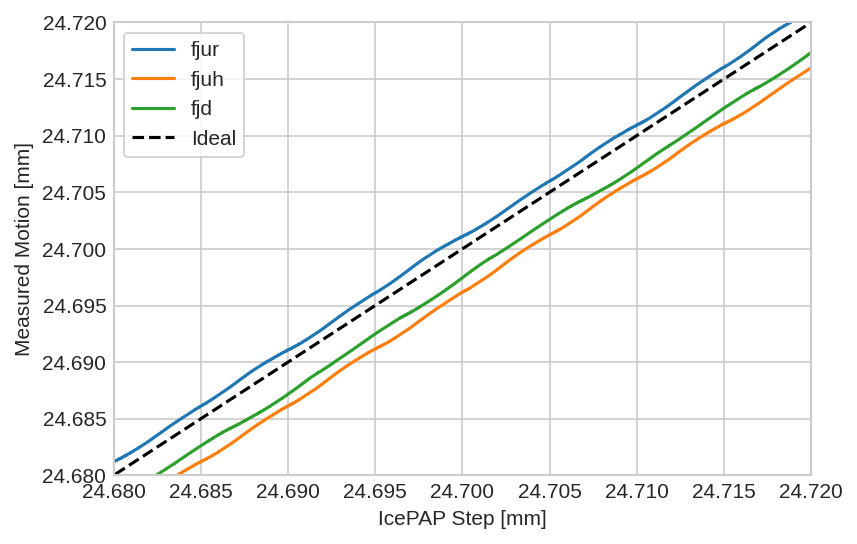
Figure 62: Measured fast jack motion as a function of the IcePAP step
5.2.4. Get Only Interesting Data
Now the data corresponding to the acceleration phase are removed.
# Remove the extreme part of the data corresponding to the acceleration phase
filt_array = np.where(np.logical_or(fjd[N_delay+1:-N_delay] > fjd[0] - 0.05e-3, fjd[N_delay+1:-N_delay] < fjd[-1] + 0.05e-3))

fjur_e_filt = np.delete(fjur_e_filt, filt_array)
fjuh_e_filt = np.delete(fjuh_e_filt, filt_array)
fjd_e_filt  = np.delete(fjd_e_filt,  filt_array)
time_filt   = np.delete(time_filt, filt_array)

fjur_filt = np.delete(fjur[N_delay+1:-N_delay], filt_array)
fjuh_filt = np.delete(fjuh[N_delay+1:-N_delay], filt_array)
fjd_filt  = np.delete(fjd[ N_delay+1:-N_delay], filt_array)
5.2.5. LUT creation
Now the LUT is initialized and computed.
# Distance bewteen LUT points in [m]
lut_inc = 100e-9
# Lut Initialization - First column is pos in [m]
lut_start = lut_inc*np.floor(np.min([[fjur_filt + fjur_e_filt], [fjuh_filt + fjuh_e_filt], [fjd_filt + fjd_e_filt]])/lut_inc)
lut_end = lut_inc*np.ceil(np.max([[fjur_filt + fjur_e_filt], [fjuh_filt + fjuh_e_filt], [fjd_filt + fjd_e_filt]])/lut_inc)

lut = np.arange(lut_start,lut_end,lut_inc)[:, np.newaxis] @ np.ones((1,4))
# Build the LUT
for i in range(0, lut.shape[0]):
    idx = (np.abs(fjur_filt + fjur_e_filt - lut[i,0])).argmin()
    if idx > 3 and idx < np.size(fjur_filt) - 3:
        lut[i,1] = fjur_filt[idx];
    idx = (np.abs(fjuh_filt + fjuh_e_filt - lut[i,0])).argmin()
    if idx > 3 and idx < np.size(fjuh_filt) - 3:
        lut[i,2] = fjuh_filt[idx];
    idx = (np.abs(fjd_filt + fjd_e_filt - lut[i,0])).argmin()
    if idx > 3 and idx < np.size(fjd_filt) - 3:
        lut[i,3] = fjd_filt[idx];
# Add points at both extremities of the LUT to make sure larger scans can be performed
# lut = np.append(lut, np.arange(lut_end+5e-6, lut_end+50e-6, 5e-6)[:, np.newaxis] @ np.ones((1,4)), axis=0)
# lut = np.insert(lut, 0, np.arange(lut_start-50e-6, lut_start-1e-6, 5e-6)[:, np.newaxis] @ np.ones((1,4)), axis=0)
lut = np.append(lut,    np.arange(lut_end+1e-3, 30e-3,     1e-3)[:, np.newaxis] @ np.ones((1,4)), axis=0)
lut = np.insert(lut, 0, np.arange(4e-3,         lut_start, 1e-3)[:, np.newaxis] @ np.ones((1,4)), axis=0)
The computed LUT is shown in Figure 63.
There is a “step” at the extremities that will slow down the scans is the steps are within the trajectories.
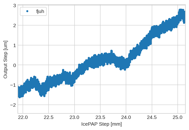
Figure 63: LUT before “normalization” of ends
In order to deal with this issue, both ends of the LUT are shifted in order to compensate this step.
# Step compensation of the start of the LUT
i = np.argmax(np.abs(lut[:,1] - lut[:,0]) > 100e-9)
ur_offset = lut[i,1] - lut[i,0]
lut[0:i,1] = lut[0:i,1] + ur_offset

i = np.argmax(np.abs(lut[:,2] - lut[:,0]) > 100e-9)
uh_offset = lut[i,2] - lut[i,0]
lut[0:i,2] = lut[0:i,2] + uh_offset

i = np.argmax(np.abs(lut[:,3] - lut[:,0]) > 100e-9)
d_offset = lut[i,3] - lut[i,0]
lut[0:i,3] = lut[0:i,3] + d_offset

# Step compensation of the end of the LUT
i = np.argmax(np.abs(lut[::-1,1] - lut[::-1,0]) > 100e-9)
ur_offset = lut[-i-1,1] - lut[-i-1,0]
lut[-i:,1] = lut[-i:,1] + ur_offset

i = np.argmax(np.abs(lut[::-1,2] - lut[::-1,0]) > 100e-9)
uh_offset = lut[-i-1,2] - lut[-i-1,0]
lut[-i:,2] = lut[-i:,2] + uh_offset

i = np.argmax(np.abs(lut[::-1,3] - lut[::-1,0]) > 100e-9)
d_offset = lut[-i-1,3] - lut[-i-1,0]
lut[-i:,3] = lut[-i:,3] + d_offset
The final LUT is displayed in Figure 64. The LUT is now smooth and trajectories larger than the LUT will be possible.
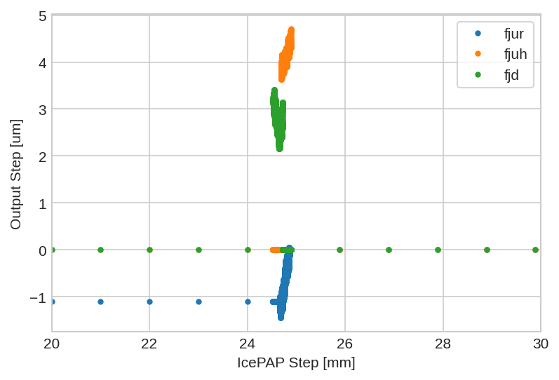
Figure 64: Figure caption
# Convert from [m] to [mm]
lut = 1e3*lut;
The LUT is saved as a .dat file that will be loaded into BLISS.
filename = "test_lut_python.dat"
print(f"Save LUT Table in {filename}")
np.savetxt(filename, lut)
5.3. New Method (Python)
In this section, the LUT is computed using Python.
5.3.1. Load Data
A scan in mode A is performed and loaded.
data = np.loadtxt("/home/thomas/mnt/data_id21/21Nov/blc13420/id21/LUT_constant_fj_vel/lut_const_fj_vel_17012022_1749.dat")
Useful data are extracted and converted to SI units.
bragg = np.pi/180*data[:,0] # Bragg Angle [rad]
dz = 1e-9*data[:,1] # Distance between crystals [m]
dry = 1e-9*data[:,2] # dry [rad]
drx = 1e-9*data[:,3] # drx [rad]
fjur = 1e-8*data[:,4] # ur Fast Jack Step in [m]
fjuh = 1e-8*data[:,5] # uh Fast Jack Step in [m]
fjd = 1e-8*data[:,6] # d Fast Jack Step in [m]
time = 1e-4*np.arange(0, np.size(bragg), 1) # Time vector [s]
ddz = 10.5e-3/(2*np.cos(bragg)) - dz; # Z error between the two crystals [m]
5.3.2. Convert Data in the frame of the fast jack
The measured motion of the crystals using the interferometers are converted to the motion of the three jacks using the Jacobian matrix.
# Actuator Jacobian
J_a_111 = np.array([[1,  0.14, -0.0675], [1,  0.14,  0.1525], [1, -0.14,  0.0425]])

# Computation of the position of the FJ as measured by the interferometers
error = J_a_111 @ [ddz, dry, drx]

fjur_e = error[0,:] # [m]
fjuh_e = error[1,:] # [m]
fjd_e  = error[2,:] # [m]
5.3.3. Filter Data
In order to get rid of external disturbances and noise, the measured fast jack displacement errors are low pass filtered.
The filter parameters are defined below.
# Generate Low pass FIR Filter
sample_rate = 10000.0 # Sample Rate [Hz]
nyq_rate = sample_rate / 2.0 # Nyquist Rate [Hz]

cutoff_hz = 27 # The cutoff frequency of the filter [Hz]

# Window with specific ripple [dB] and width [Nyquist Fraction]
N, beta = kaiserord(60, 4/nyq_rate)

# Delay expressed in number of sample
N_delay = int((N-1)/2)

# Delay expressed in seconds
delay = N_delay / sample_rate
The filter is generated using the following command:
# Fitler generation
taps = firwin(N, cutoff_hz/nyq_rate, window=('kaiser', beta))
This filter will introduce a constant delay that is a function of its length:
print("Length of the filter is %i\nDelay is %i samples (i.e. %.3f seconds)" % (N, N_delay, delay))
Length of the filter is 9065
Delay is 4532 samples (i.e. 0.453 seconds)
The measured data is then filtered using the lfilter command.
The obtained raw and filtered data are displayed in Figure 61.
# Filtering of data, compensation of the delay introduced by the FIR filter
fjur_e_filt = lfilter(taps, 1.0, fjur_e)[N:]
fjuh_e_filt = lfilter(taps, 1.0, fjuh_e)[N:]
fjd_e_filt = lfilter(taps, 1.0, fjd_e)[N:]
time_filt = time[N_delay+1:-N_delay]
The measured fast jack motion (filtered) as a function of the IcePAP steps (desired position) is shown in Figure 62 for the three fast jacks.
Figure 65: Measured fast jack motion as a function of the IcePAP step
5.3.4. Get Only Interesting Data
Now the data corresponding to the acceleration phase are removed.
# Remove the extreme part of the data corresponding to the acceleration phase
filt_array = np.where(np.logical_or(fjd[N_delay+1:-N_delay] > fjd[0] - 0.05e-3, fjd[N_delay+1:-N_delay] < fjd[-1] + 0.05e-3))

fjur_e_filt = np.delete(fjur_e_filt, filt_array)
fjuh_e_filt = np.delete(fjuh_e_filt, filt_array)
fjd_e_filt  = np.delete(fjd_e_filt,  filt_array)
time_filt   = np.delete(time_filt, filt_array)

fjur_filt = np.delete(fjur[N_delay+1:-N_delay], filt_array)
fjuh_filt = np.delete(fjuh[N_delay+1:-N_delay], filt_array)
fjd_filt  = np.delete(fjd[ N_delay+1:-N_delay], filt_array)
5.3.5. New LUT creation
u, c = np.unique(fjur_filt, return_index=True)
lut_ur = np.stack((u + fjur_e_filt[c], u))

u, c = np.unique(fjuh_filt, return_index=True)
lut_uh = np.transpose(np.stack((u + fjuh_e_filt[c], u)))

u, c = np.unique(fjd_filt, return_index=True)
lut_d = np.transpose(np.stack((u + fjd_e_filt[c], u)))
# Figure - Correction made by the new LUT
plt.figure(figsize=(1200/150, 800/150), dpi=150)
plt.clf
plt.plot(1e3*lut_ur[:,0], 1e6*(lut_ur[:,1] - lut_ur[:,0]), '.', label='fjur')
plt.plot(1e3*lut_uh[:,0], 1e6*(lut_uh[:,1] - lut_uh[:,0]), '.', label='fjuh')
plt.plot(1e3*lut_d[:,0], 1e6*(lut_d[:,1] - lut_d[:,0]), '.', label='fjd')
plt.xlabel('IcePAP Step [mm]')
plt.ylabel('Output Step [um]')
plt.legend(frameon=True)
plt.xlim([24.5, 24.9])
plt.savefig('figs/python_new_lut.pdf', transparent=True, bbox_inches='tight', pad_inches=0)
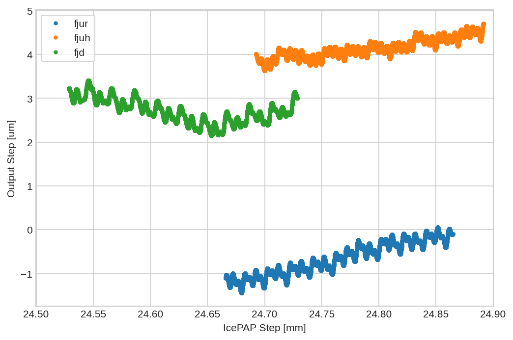
Figure 66: Correction made by the new LUT
# Figure - Correction made by the new LUT
plt.figure(figsize=(1200/150, 800/150), dpi=150)
plt.clf
plt.plot(1e3*lut_ur[:,0], 1e6*(lut_ur[:,1] - lut_ur[:,0]), '.', label='fjur')
plt.plot(1e3*lut[:,0], 1e6*(lut[:,1] - lut[:,0]), '.', label='fjur')
plt.xlabel('IcePAP Step [mm]')
plt.ylabel('Output Step [um]')
plt.legend(frameon=True)
plt.xlim([24.7, 24.71])
plt.ylim([-1.4, -0.8])
plt.savefig('figs/python_new_lut.pdf', transparent=True, bbox_inches='tight', pad_inches=0)
5.3.6. LUT creation
Now the LUT is initialized and computed.
# Distance bewteen LUT points in [m]
lut_inc = 100e-9
# Lut Initialization - First column is pos in [m]
lut_start = lut_inc*np.floor(np.min([[fjur_filt + fjur_e_filt], [fjuh_filt + fjuh_e_filt], [fjd_filt + fjd_e_filt]])/lut_inc)
lut_end = lut_inc*np.ceil(np.max([[fjur_filt + fjur_e_filt], [fjuh_filt + fjuh_e_filt], [fjd_filt + fjd_e_filt]])/lut_inc)

lut = np.arange(lut_start,lut_end,lut_inc)[:, np.newaxis] @ np.ones((1,4))
# Build the LUT
for i in range(0, lut.shape[0]):
    idx = (np.abs(fjur_filt + fjur_e_filt - lut[i,0])).argmin()
    if idx > 3 and idx < np.size(fjur_filt) - 3:
        lut[i,1] = fjur_filt[idx];
    idx = (np.abs(fjuh_filt + fjuh_e_filt - lut[i,0])).argmin()
    if idx > 3 and idx < np.size(fjuh_filt) - 3:
        lut[i,2] = fjuh_filt[idx];
    idx = (np.abs(fjd_filt + fjd_e_filt - lut[i,0])).argmin()
    if idx > 3 and idx < np.size(fjd_filt) - 3:
        lut[i,3] = fjd_filt[idx];
# Add points at both extremities of the LUT to make sure larger scans can be performed
# lut = np.append(lut, np.arange(lut_end+5e-6, lut_end+50e-6, 5e-6)[:, np.newaxis] @ np.ones((1,4)), axis=0)
# lut = np.insert(lut, 0, np.arange(lut_start-50e-6, lut_start-1e-6, 5e-6)[:, np.newaxis] @ np.ones((1,4)), axis=0)
lut = np.append(lut,    np.arange(lut_end+1e-3, 30e-3,     1e-3)[:, np.newaxis] @ np.ones((1,4)), axis=0)
lut = np.insert(lut, 0, np.arange(4e-3,         lut_start, 1e-3)[:, np.newaxis] @ np.ones((1,4)), axis=0)
The computed LUT is shown in Figure 63.
There is a “step” at the extremities that will slow down the scans is the steps are within the trajectories.
Figure 67: LUT before “normalization” of ends
In order to deal with this issue, both ends of the LUT are shifted in order to compensate this step.
# Step compensation of the start of the LUT
i = np.argmax(np.abs(lut[:,1] - lut[:,0]) > 100e-9)
ur_offset = lut[i,1] - lut[i,0]
lut[0:i,1] = lut[0:i,1] + ur_offset

i = np.argmax(np.abs(lut[:,2] - lut[:,0]) > 100e-9)
uh_offset = lut[i,2] - lut[i,0]
lut[0:i,2] = lut[0:i,2] + uh_offset

i = np.argmax(np.abs(lut[:,3] - lut[:,0]) > 100e-9)
d_offset = lut[i,3] - lut[i,0]
lut[0:i,3] = lut[0:i,3] + d_offset

# Step compensation of the end of the LUT
i = np.argmax(np.abs(lut[::-1,1] - lut[::-1,0]) > 100e-9)
ur_offset = lut[-i-1,1] - lut[-i-1,0]
lut[-i:,1] = lut[-i:,1] + ur_offset

i = np.argmax(np.abs(lut[::-1,2] - lut[::-1,0]) > 100e-9)
uh_offset = lut[-i-1,2] - lut[-i-1,0]
lut[-i:,2] = lut[-i:,2] + uh_offset

i = np.argmax(np.abs(lut[::-1,3] - lut[::-1,0]) > 100e-9)
d_offset = lut[-i-1,3] - lut[-i-1,0]
lut[-i:,3] = lut[-i:,3] + d_offset
The final LUT is displayed in Figure 64. The LUT is now smooth and trajectories larger than the LUT will be possible.
Figure 68: Figure caption
# Convert from [m] to [mm]
lut = 1e3*lut;
The LUT is saved as a .dat file that will be loaded into BLISS.
filename = "test_lut_python.dat"
print(f"Save LUT Table in {filename}")
np.savetxt(filename, lut)
5.3.7. Merge LUT
lut_ur = np.transpose(np.loadtxt("/home/thomas/mnt/data_id21/tmp/LUT_full_new_ur.dat"))
lut_uh = np.transpose(np.loadtxt("/home/thomas/mnt/data_id21/tmp/LUT_full_new_uh.dat"))
lut_d = np.transpose(np.loadtxt("/home/thomas/mnt/data_id21/tmp/LUT_full_new_d.dat"))
merge_1 = (lut_1_ur[0,-1]+lut_2_ur[0,0])/2
merge_2 = (lut_2_ur[0,-1]+lut_3_ur[0,0])/2
lut_ur = np.concatenate((
    lut_1_ur[:, lut_1_ur[0,:] < merge_1],
    lut_2_ur[:, np.logical_and(lut_2_ur[0,:] > merge_1, lut_2_ur[0,:] < merge_2)],
    lut_3_ur[:, lut_3_ur[0,:] > merge_2]
), axis=1)
6. Optimal Trajectory
In this section, the problem of generating an adequate trajectory to make the LUT is studied.
The problematic is the following:
- the positioning errors of the fast jack should be measured
- all external disturbances and measurement noise should be filtered out.
The main difficulty is that the frequency of both the positioning errors errors and the disturbances are a function of the scanning velocity.
First, the frequency of the disturbances as well as the errors to be measured are described and a filter is designed to optimally separate disturbances from positioning errors (Section 6). The relation between the Bragg angular velocity and fast jack velocity is studied in Section 6.2. Next, a trajectory with constant fast jack velocity (Section 6.3) and with constant Bragg angular velocity (Section 6.4) are simulated to understand their limitations. Finally, it is proposed to perform a scan in two parts (one part with constant fast jack velocity and the other part with constant bragg angle velocity) in Section 6.5.
6.1. Filtering Disturbances and Noise
Based on measurements made in mode A (without LUT or feedback control), several disturbances could be identified:
- vibrations coming from from the
mcoilmotor - vibrations with constant frequencies at 29Hz (pump), 34Hz (air conditioning) and 45Hz (un-identified)
These disturbances as well as the noise of the interferometers should be filtered out, and only the fast jack motion errors should be left untouched.
Therefore, the goal is to make a scan such that during all the scan, the frequencies of the errors induced by the fast jack have are smaller than the frequencies of all other disturbances. Then, it is easy to use a filter to separate the disturbances and noise from the positioning errors of the fast jack.
6.1.0.1. Errors induced by the Fast Jack
The Fast Jack is composed of one stepper motor, and a planetary roller screw with a pitch of 1mm/turn. The stepper motor as 50 pairs of magnetic poles, and therefore positioning errors are to be expected every 1/50th of turn (and its harmonics: 1/100th of turn, 1/200th of turn, etc.).
One pair of magnetic pole corresponds to an axial motion of \(20\,\mu m\). Therefore, errors are to be expected with a period of \(20\,\mu m\) and harmonics at \(10\,\mu m\), \(5\,\mu m\), \(2.5\,\mu m\), etc.
As the LUT has one point every \(1\,\mu m\), we wish to only measure errors with a period of \(20\,\mu m\), \(10\,\mu m\) and \(5\,\mu m\). Indeed, errors with smaller periods are small in amplitude (i.e. not worth to compensate) and are difficult to model with the limited number of points in the LUT.
The frequency corresponding to errors with a period of \(5\,\mu m\) at 1mm/s is:
Frequency or errors with period of 5um/s at 1mm/s is: 200.0 [Hz]
We wish that the frequency of the error corresponding to a period of \(5\,\mu m\) to be smaller than the smallest disturbance to be filtered.
As the main disturbances are at 34Hz and 45Hz, we constrain the the maximum axial velocity of the Fast Jack such that the positioning error has a frequency bellow 25Hz:
max_fj_vel = 25*1e-3/(1e-3/5e-6); % [m/s]
Maximum Fast Jack velocity: 0.125 [mm/s]
Therefore, the Fast Jack scans should be scanned at rather low velocity for the positioning errors to be at sufficiently low frequency.
6.1.0.2. Vibrations induced by mcoil
The mcoil system is composed of one stepper motor and a reducer such that one stepper motor turns makes the mcoil axis to rotate 0.2768 degrees.
When scanning the mcoil motor, periodic vibrations can be measured by the interferometers.
It has been identified that the period of these vibrations are corresponding to the period of the magnetic poles (50 per turn as for the Fast Jack stepper motors).
Therefore, the frequency of these periodic errors are a function of the angular velocity. With an angular velocity of 1deg/s, the frequency of the vibrations are expected to be at:
Fundamental frequency at 1deg/s: 180.6 [Hz]
We wish the frequency of these errors to be at minimum 34Hz (smallest frequency of other disturbances).
The corresponding minimum mcoil velocity is:
min_bragg_vel = 34/(50/0.2768); % [deg/s]
Min mcoil velocity is 0.19 [deg/s]
Regarding the mcoil motor, the problematic is to not scan too slowly.
It should however be checked whether the amplitude of the induced vibrations is significant of not.
Note that the maximum bragg angular velocity is:
max_bragg_vel = 1; % [deg/s]
6.1.0.3. Measurement noise of the interferometers
The motion of the fast jacks are measured by interferometers which have some measurement noise. It is wanted to filter this noise to acceptable values to have a clean measured position.
As the interferometer noise has a rather flat spectral density, it is easy to estimate its RMS value as a function of the cut-off frequency of the filter.
The RMS value of the filtered interferometer signal as a function of the cutoff frequency of the low pass filter is computed and shown in Figure 69.
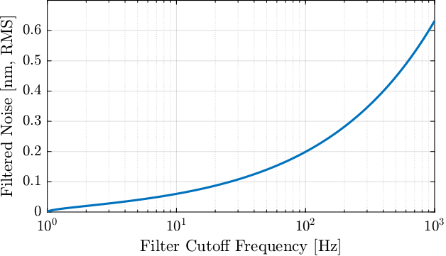
Figure 69: Filtered noise RMS value as a function of the low pass filter cut-off frequency
As the filter will have a cut-off frequency between 25Hz (maximum frequency of the positioning errors) and 34Hz (minimum frequency of disturbances), a filtered measurement noise of 0.1nm RMS is to be expected.
Figure 69 is a rough estimate. Precise estimation can be done by measuring the spectral density of the interferometer noise experimentally.
6.1.0.4. Interferometer - Periodic non-linearity
Interferometers can also show periodic non-linearity with a (fundamental) period equal to half the wavelength of its light (i.e. 765nm for Attocube) and with unacceptable amplitudes (up to tens of nanometers).
The minimum frequency associated with these errors is therefore a function of the fast jack velocity. With a velocity of 1mm/s, the frequency is:
Fundamental frequency at 1mm/s: 1307.2 [Hz]
We wish these errors to be at minimum 34Hz (smallest frequency of other disturbances). The corresponding minimum velocity of the Fast Jack is:
min_fj_vel = 34*1e-3/(1e-3/765e-9); % [m/s]
Minimum Fast Jack velocity is 0.026 [mm/s]
The Fast Jack Velocity should not be too low or the frequency of the periodic non-linearity of the interferometer would be too small to be filtered out (i.e. in the pass-band of the filter).
6.1.0.5. Implemented Filter
Let’s now verify that it is possible to implement a filter that keep everything untouched below 25Hz and filters everything above 34Hz.
To do so, a FIR linear phase filter is designed:
%% FIR with Linear Phase
Fs = 1e4; % Sampling Frequency [Hz]
B_fir = firls(5000, ... % Filter's order
              [0 25/(Fs/2) 34/(Fs/2) 1], ... % Frequencies [Hz]
              [1 1          0          0]); % Wanted Magnitudes
Its amplitude response is shown in Figure 70. It is confirmed that the errors to be measured (below 25Hz) are left untouched while the disturbances above 34Hz are reduced by at least a factor \(10^4\).
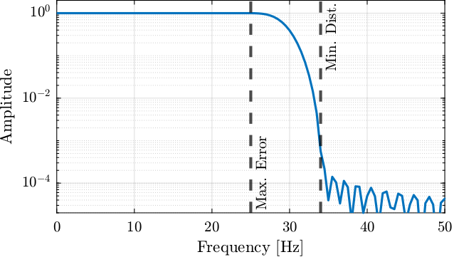
Figure 70: FIR filter’s response
To have such a steep change in gain, the order of the filter is rather large. This has the negative effect of inducing large time delays:
Induced time delay is 0.25 [s]
This time delay is only requiring us to start the acquisition 0.25 seconds before the important part of the scan is performed (i.e. the first 0.25 seconds of data cannot be filtered).
6.2. First Estimation of the optimal trajectory
Based on previous analysis (Section 6.1), minimum and maximum fast jack velocities and bragg angular velocities could be determined. These values are summarized in Table 4. Therefore, if during the scan the velocities are within the defined bounds, it will be very easy to filter the data and extract only the relevant information (positioning error of the fast jack).
| Min | Max | |
|---|---|---|
| Bragg Angular Velocity [deg/s] | 0.188 | 1.0 |
| Fast Jack Velocity [mm/s] | 0.026 | 0.125 |
We now wish to see if it is possible to perform a scan from 5deg to 75deg of bragg angle while keeping the velocities within the bounds in Table 4.
To study that, we can compute the relation between the Bragg angular velocity and the Fast Jack velocity as a function of the Bragg angle.
To do so, we first look at the relation between the Bragg angle \(\theta_b\) and the Fast Jack position \(d_{\text{FJ}}\):
\begin{equation} d_{FJ}(t) = d_0 - \frac{10.5 \cdot 10^{-3}}{2 \cos \theta_b(t)} \end{equation}with \(d_0 \approx 0.030427\,m\).
Then, by taking the time derivative, we obtain the relation between the Fast Jack velocity \(\dot{d}_{\text{FJ}}\) and the Bragg angular velocity \(\dot{\theta}_b\) as a function of the bragg angle \(\theta_b\):
\begin{equation} \label{eq:bragg_angle_formula} \boxed{\dot{d}_{FJ}(t) = - \dot{\theta_b}(t) \cdot \frac{10.5 \cdot 10^{-3}}{2} \cdot \frac{\tan \theta_b(t)}{\cos \theta_b(t)}} \end{equation}The relation between the Bragg angular velocity and the Fast Jack velocity is computed for several angles starting from 5degrees up to 75 degrees and this is shown in Figure 71.
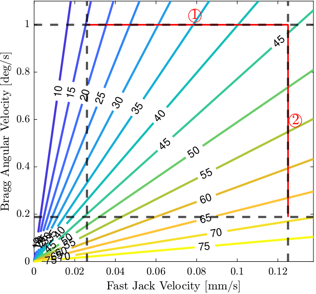
Figure 71: Bragg angular velocity as a function of the fast jack velocity for several bragg angles (indicated by the colorful lines in degrees). Black dashed lines indicated minimum/maximum bragg angular velocities as well as minimum/maximum fast jack velocities
From Figure 71, it is clear that only Bragg angles from apprimately 15 to 70 degrees can be scanned by staying in the “perfect” zone (defined by the dashed black lines).
To scan smaller bragg angles, either the maximum bragg angular velocity should be increased or the minimum fast jack velocity decreased (accepting some periodic non-linearity to be measured).
To scan higher bragg angle, either the maximum fast jack velocity should be increased or the minimum bragg angular velocity decreased (taking the risk to have some disturbances from the mcoil motion in the signal).
For Bragg angles between 15 degrees and 70 degrees, several strategies can be chosen:
- Constant Fast Jack velocity (Figure 72 - Left):
- Go from 15 degrees to 44 degrees at minimum fast jack velocity
- Go from 44 degrees to 70 degrees at maximum fast jack velocity
- Constant Bragg angular velocity (Figure 72 - Right):
- Go from 15 degrees to 44 degrees at maximum angular velocity
- Go from 44 to 70 degrees at minimum angular velocity
- A mixed of constant bragg angular velocity and constant fast jack velocity (Figure 71 - Red line)
- from 15 to 44 degrees with maximum Bragg angular velocity
- from 44 to 70 degrees with maximum Bragg angular velocity
The third option is studied in Section 6.4
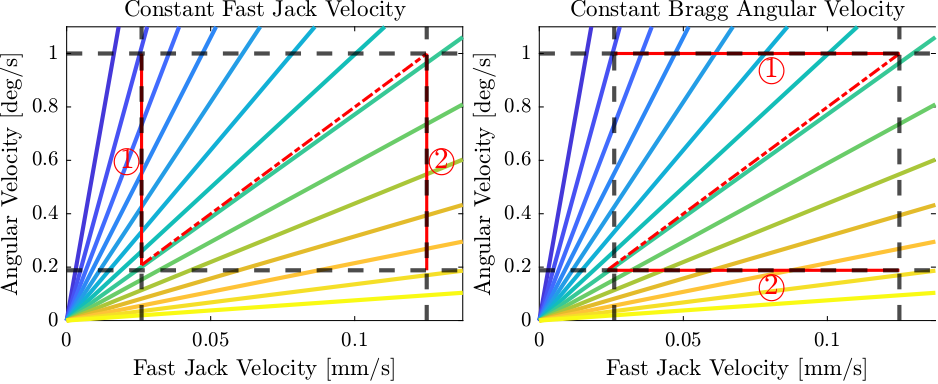
Figure 72: Angular velocity and fast jack velocity during two scans from 5 to 75 degrees. On the left for a scan with constant fast jack velocity. On the right for a scan with constant Bragg angular velocity.
6.3. Constant Fast Jack Velocity
In this section, a scan with constant fast jack velocity is studied.
It was shown in Section 6 that the maximum Fast Jack velocity should be 0.125mm/s in order for the frequency corresponding to the period of \(5\,\mu m\) to be smaller than 25Hz.
Let’s generate a trajectory between 5deg and 75deg Bragg angle with constant Fast Jack velocity at 0.125mm/s.
%% Compute extreme fast jack position
fj_max = 0.030427 - 10.5e-3/(2*cos(pi/180*5)); % Smallest FJ position [m]
fj_min = 0.030427 - 10.5e-3/(2*cos(pi/180*75)); % Largest FJ position [m]

%% Compute Fast Jack Trajectory
t = 0:0.1:(fj_max - fj_min)/max_fj_vel; % Time vector [s]
fj_pos = fj_max - t*max_fj_vel; % Fast Jack Position [m]

%% Compute corresponding Bragg trajectory
bragg_pos = acos(10.5e-3./(2*(0.030427 - fj_pos))); % [rad]
The Fast Jack position as well as the Bragg angle are shown as a function of time in Figure 73.
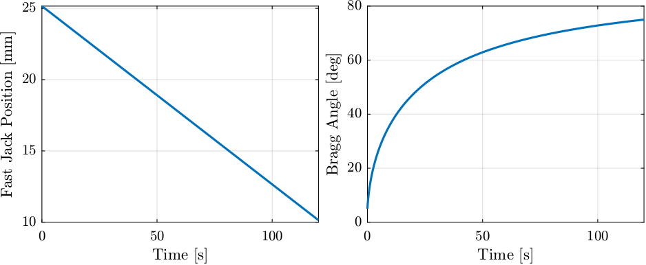
Figure 73: Trajectory with constant Fast Jack Velocity
Let’s now compute the Bragg angular velocity for this scan (Figure 74). It is shown that for large Fast Jack positions / small bragg angles, the bragg angular velocity is too large.
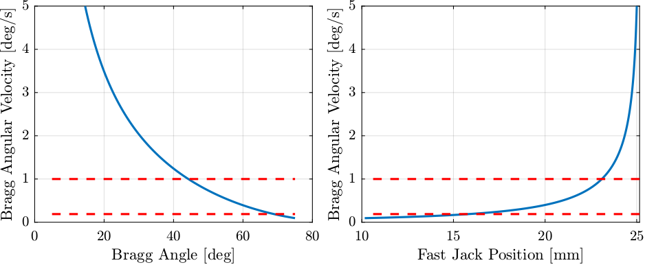
Figure 74: Bragg Velocity as a function of the bragg angle or fast jack position
Between 45 and 70 degrees, the scan can be performed with constant Fast Jack velocity equal to 0.125 mm/s.
6.4. Constant Bragg Angular Velocity
Let’s now study a scan with a constant Bragg angular velocity of 1deg/s.
%% Time vector for the Scan with constant angular velocity
t = 0:0.1:(75 - 5)/max_bragg_vel; % Time vector [s]

%% Bragg angle during the scan
bragg_pos = 5 + t*max_bragg_vel; % Bragg Angle [deg]

%% Computation of the Fast Jack Position
fj_pos = 0.030427 - 10.5e-3./(2*cos(pi/180*bragg_pos)); % FJ position [m]
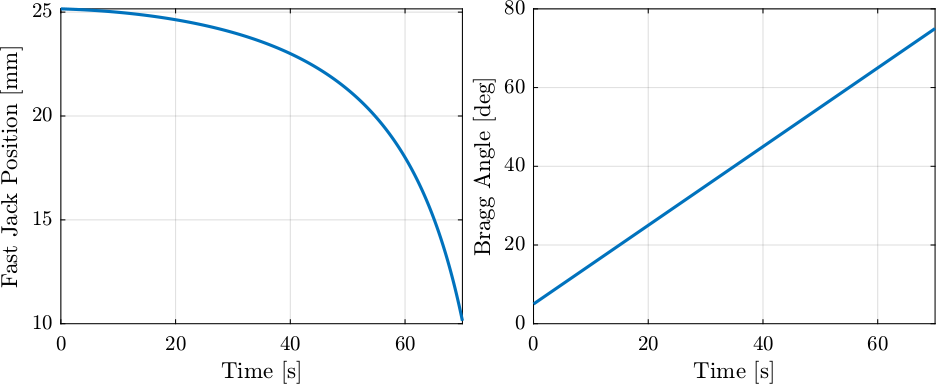
Figure 75: Trajectory with constant Bragg angular velocity
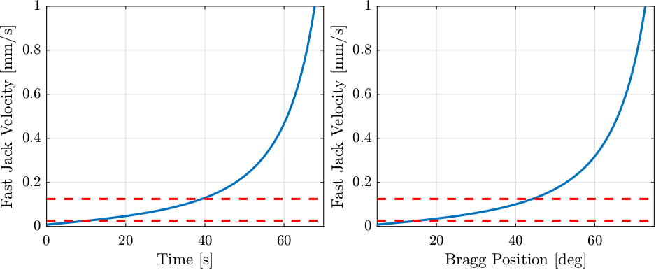
Figure 76: Fast Jack Velocity with a constant bragg angular velocity
Between 15 and 45 degrees, the scan can be performed with a constant Bragg angular velocity equal to 1 deg/s.
6.5. Mixed Trajectory
Let’s combine a scan with constant Bragg angular velocity for small bragg angles (< 44.3 deg) with a scan with constant Fast Jack velocity for large Bragg angle (> 44.3 deg). The scan is performed from 5 degrees to 75 degrees.
Parameters for the scan are defined below:
%% Bragg Positions
bragg_start = 5; % Start Bragg angle [deg]
bragg_mid   = 44.3; % Transition between constant FJ vel and constant Bragg vel [deg]
bragg_end   = 75; % End Bragg angle [deg]

%% Fast Jack Positions
fj_start = 0.030427 - 10.5e-3/(2*cos(pi/180*bragg_start)); % Start FJ position [m]
fj_mid   = 0.030427 - 10.5e-3/(2*cos(pi/180*bragg_mid)); % Mid FJ position [m]
fj_end   = 0.030427 - 10.5e-3/(2*cos(pi/180*bragg_end)); % End FJ position [m]

%% Time vectors
Ts = 0.1; % Sampling Time [s]
t_c_bragg = 0:Ts:(bragg_mid-bragg_start)/max_bragg_vel; % Time Vector for constant bragg velocity [s]
t_c_fj = Ts+[0:Ts:(fj_mid-fj_end)/max_fj_vel]; % Time Vector for constant Fast Jack velocity [s]
Positions for the first part of the scan at constant Bragg angular velocity are computed:
%% Constant Bragg Angular Velocity
bragg_c_bragg = bragg_start + t_c_bragg*max_bragg_vel; % [deg]
fj_c_bragg = 0.030427 - 10.5e-3./(2*cos(pi/180*bragg_c_bragg)); % FJ position [m]
And positions for the part of the scan with constant Fast Jack Velocity are computed:
%% Constant Bragg Angular Velocity
fj_c_fj = fj_mid - t_c_fj*max_fj_vel; % FJ position [m]
bragg_c_fj = 180/pi*acos(10.5e-3./(2*(0.030427 - fj_c_fj))); % [deg]
Fast Jack position as well as Bragg angle are displayed as a function of time in Figure 77.
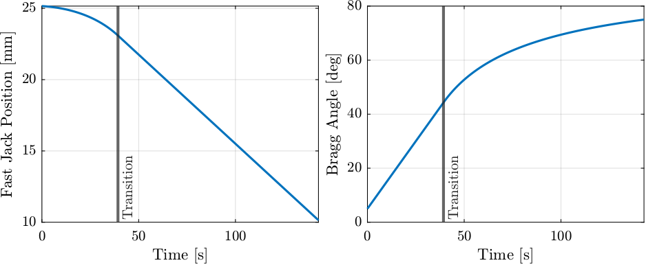
Figure 77: Fast jack trajectories and Bragg angular velocity during the scan
The Fast Jack velocity as well as the Bragg angular velocity are shown as a function of the Bragg angle in Figure 78.
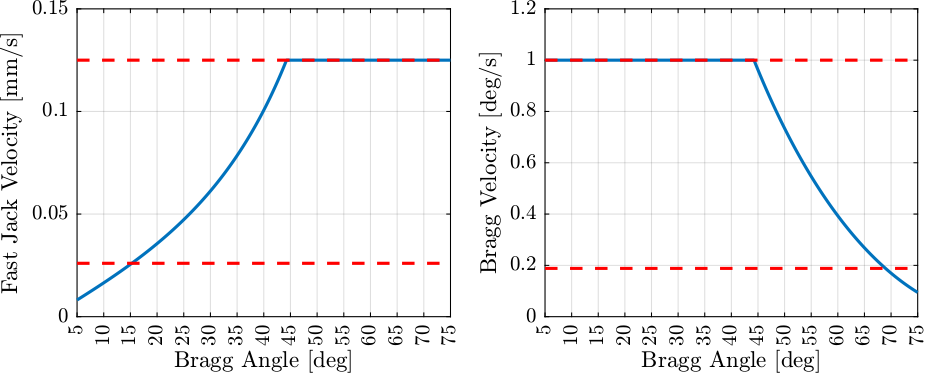
Figure 78: Fast jack velocity and Bragg angular velocity during the scan
From Figure 78, it is shown that the fast jack velocity as well as the bragg angular velocity are within the bounds except:
- Below 15 degrees where the fast jack velocity is too small. The frequency of the non-linear periodic errors of the interferometers would be at too low frequency (in the pass-band of the filter, see Figure 79). One easy option is to use an interferometer without periodic non-linearity. Another option is to increase the maximum Bragg angular velocity to 3 deg/s.
- Above 70 degrees where the Bragg angular velocity is too small.
This may introduce low frequency disturbances induced by the
mcoilmotor that would be in the pass-band of the filter (see Figure 79). It should be verified if this is indeed problematic of not. An other way would be to scan without themcoilmotor at very high bragg angle.
In order to better visualize the filtering problem, the frequency of all the signals are shown as a function of the Bragg angle during the scan in Figure 79.
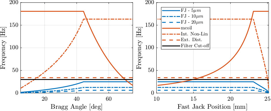
Figure 79: Frequency of signals as a function of the Bragg angle and Fast Jack position
7. Constant Fast Jack velocity
A new trajectory motor fjstraj has been created to be able to perform scans with constant Fast Jack velocity.
As explained in Section 6, this can help with the filtering of the data as positioning errors with periods of \(5\,\mu m\), \(10\,\mu m\) and \(20\,\mu m\) will be seen with a constant frequency in the time domain. The frequency of these errors can be tuned by properly choosing the fast jack velocity.
7.1. Analysis of measured motion
In this section, a scan with constant fast jack velocity is performed and the measurements are analyzed.
The measurements data are loaded and converted to SI units (mostly meters and radians). Bragg and Fast Jack velocity are computed and shown in Figure 80. We can see that during the scan, the fast jack velocity is constant and equal to \(0.125\,mm/s\) while the bragg velocity is increasing.
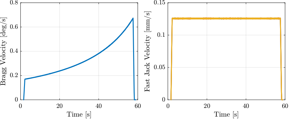
Figure 80: Bragg and Fast Jack velocity
The frequency of the measured motion errors on fjur are computed as a function a time (spectrogram) and shown in Figure 81.
The vibrations linked to the motion of the bragg angle (more precisely due to mcoil motor) are clearly observed (purple lines).
The motion errors of the fast jacks have a constant frequency.
The frequency corresponding to the error period of \(5\,\mu m\) is indicated by the dashed black line.
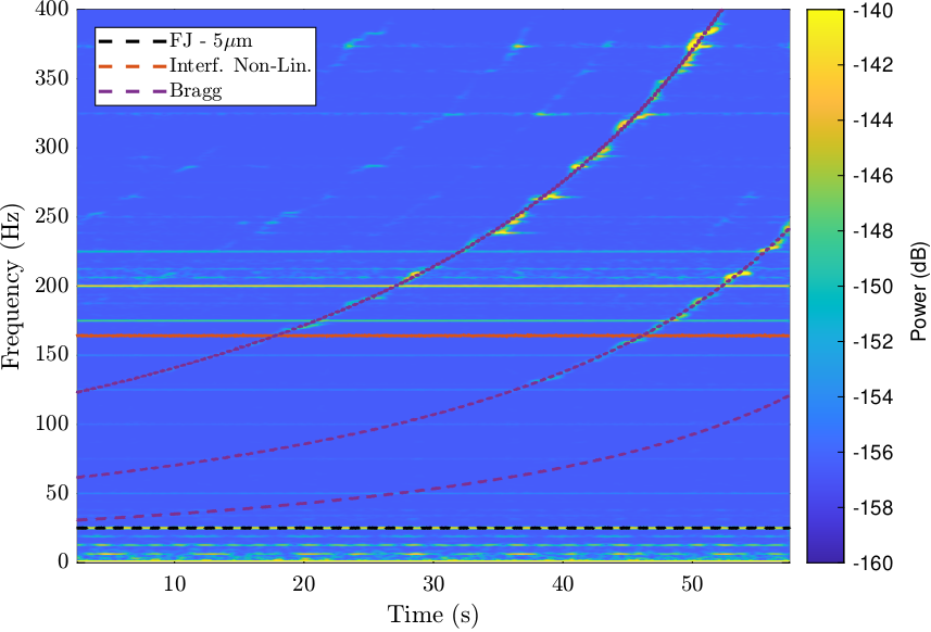
Figure 81: Spectrogram of fjsuh during the constant Fast Jack velocity scan. Bragg (mcoil motor) disturbances can clearly by seen above 150Hz and they not seems to be a problem at low Bragg velocity.
The (raw) measured positions of each fast jack are displayed as a function of the wanted position (i.e. IcePAP steps) in Figure 82. It is clear that there are some high frequency vibrations/disturbances that are making the relation between the measured position and the wanted position not bijective.
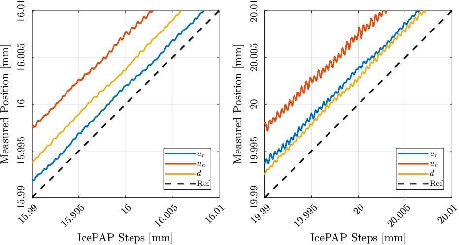
Figure 82: IcePAP steps and measured position during the scan with constant Fast Jack velocity
The data is then filtered with a sharp low pass filter that filters everything above 30Hz such that the motion errors of the fast jacks are left untouched and all other disturbances are well attenuated. The results are shown in Figure 83 where it is clear that the relation between the measured motion and the wanted motion is now a bijective function.
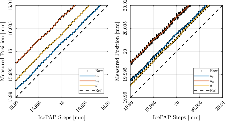
Figure 83: IcePAP steps and measured position during the scan with constant Fast Jack velocity. Comparison of the raw and filtered data.
If we only look at the measured position error of the fast jack (i.e. measured position minus the wanted position/IcePAP steps), we obtain the data of Figure 84.
The errors with a period of \(5\,\mu m\) can be clearly observed.
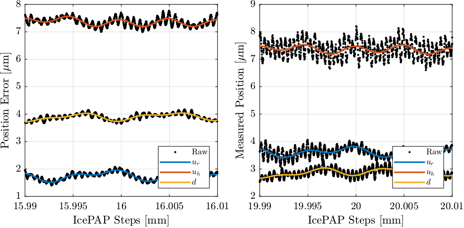
Figure 84: Raw and filtered measured position errors during the scan with constant Fast Jack velocity
7.2. LUT Creation
A Lookup Table is now computed from the filtered data with a point every \(100\,nm\) of fast jack motion.
%% Generate LUT
createLUT(data_A, "lut/lut_const_fj_vel_12012022_1139.dat", "lut_inc", 100e-9);
The obtained lookup table is displayed in Figure 85.
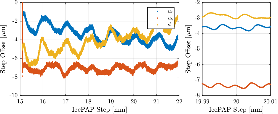
Figure 85: Obtained Lookup Table data
7.3. Comparison of errors in mode A and mode B
The Lookup Table is loaded in the IcePAP and a new scan is performed.
The measured position errors of the fast jacks are compared for the scan in mode A and in mode B in Figure 86.
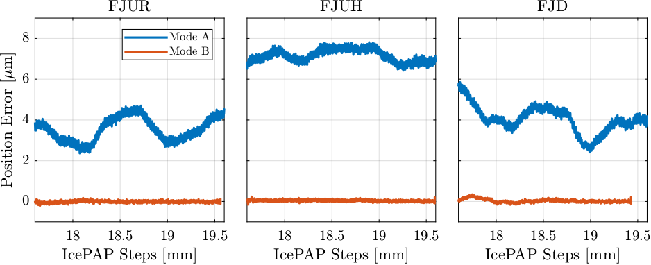
Figure 86: Comparison of the measured fast jack position errors in mode A and mode B
7.4. Test LUT just after making it
%% Generate LUT
createLUT(data_A, "matlab/lut/lut_data_const_fj_vel_14012022_1720.dat", "lut_inc", 100e-9);
scp matlab/lut/lut_data_const_fj_vel_14012022_1720.dat opid21@lid21nano:/users/blissadm/local/beamline_configuration/DCM/CALIB/LUT/
%% Load the generated LUT
data_lut = importdata("lut_data_const_fj_vel_14012022_1720.dat");
data_files = {
    "lut_const_fj_vel_14012022_1725.dat",
    "lut_const_fj_vel_14012022_1726.dat",
    "lut_const_fj_vel_14012022_1727.dat",
    "lut_const_fj_vel_14012022_1728.dat",
    "lut_const_fj_vel_14012022_1730.dat"
};
data_400nm = {};

for i = 1:length(data_files)
    data_400nm{i} = extractDatData(sprintf("%s/21Nov/blc13420/id21/LUT_constant_fj_vel/%s", data_directory, data_files{i}), ...
                         {"bragg", "dz", "dry", "drx", "fjur", "fjuh", "fjd"}, ...
                         [pi/180, 1e-9, 1e-9, 1e-9, 1e-8, 1e-8, 1e-8]);

    data_400nm{i}.ddz  = 10.5e-3./(2*cos(data_400nm{i}.bragg)) - data_400nm{i}.dz;
    data_400nm{i}.time = 1e-4*[1:1:length(data_400nm{i}.bragg)];

    %% Computation of the position of the FJ as measured by the interferometers
    error = J_a_111 * [data_400nm{i}.ddz, data_400nm{i}.dry, data_400nm{i}.drx]';

    data_400nm{i}.fjur_e = error(1,:)'; % [m]
    data_400nm{i}.fjuh_e = error(2,:)'; % [m]
    data_400nm{i}.fjd_e  = error(3,:)'; % [m]

    %% Filtering all measured Fast Jack Position using the FIR filter
    data_400nm{i}.fjur_e_filt = filter(B_fir, 1, data_400nm{i}.fjur_e);
    data_400nm{i}.fjuh_e_filt = filter(B_fir, 1, data_400nm{i}.fjuh_e);
    data_400nm{i}.fjd_e_filt  = filter(B_fir, 1, data_400nm{i}.fjd_e);

    %% Compensation of the delay introduced by the FIR filter
    data_400nm{i}.fjur_e_filt(1:end-delay) = data_400nm{i}.fjur_e_filt(delay+1:end);
    data_400nm{i}.fjuh_e_filt(1:end-delay) = data_400nm{i}.fjuh_e_filt(delay+1:end);
    data_400nm{i}.fjd_e_filt( 1:end-delay) = data_400nm{i}.fjd_e_filt( delay+1:end);
end
%% Re-sample data to have same data points in FJUR
for i = 1:length(data_files)
    [data_400nm{i}.fjur_e_resampl, data_400nm{i}.fjur_resampl] = resample(data_400nm{i}.fjur_e_filt, data_400nm{i}.fjur, 1/100e-9);
    [data_400nm{i}.fjuh_e_resampl, data_400nm{i}.fjuh_resampl] = resample(data_400nm{i}.fjuh_e_filt, data_400nm{i}.fjuh, 1/100e-9);
    [data_400nm{i}.fjd_e_resampl, data_400nm{i}.fjd_resampl] = resample(data_400nm{i}.fjd_e_filt, data_400nm{i}.fjd, 1/100e-9);
end
%% Mean Motion
fjur_400nm_e_mean = mean(cell2mat(cellfun(@(x) x.fjur_e_resampl, data_400nm, "UniformOutput", false)), 2);
fjuh_400nm_e_mean = mean(cell2mat(cellfun(@(x) x.fjuh_e_resampl, data_400nm, "UniformOutput", false)), 2);
fjd_400nm_e_mean = mean(cell2mat(cellfun(@(x) x.fjd_e_resampl, data_400nm, "UniformOutput", false)), 2);
%% Compute RMS error in mode B with LUT every 400nmm
fjur_400nm_rms = 1e9*mean(cellfun(@(x) rms(detrend(x.fjur_e_resampl - fjur_e_mean, 0)), data_400nm))
FJUR = 76.2 [nm, RMS] in mode B after several minutes (1 um LUT increment)
Repeatable Part:
7.5. Make a LUT based on mode B
%% Generate LUT
createLUT(data_A, "matlab/lut/lut_data_bis_const_fj_vel_14012022_1720.dat", "lut_inc", 100e-9);
data_lut_1 = importdata("lut_data_const_fj_vel_14012022_1720.dat");
data_lut_2 = importdata("lut_data_bis_const_fj_vel_14012022_1720.dat");
Update the LUT:
fj_start = max([data_lut_1(1,1), data_lut_2(1,1)]);
fj_end = min([data_lut_1(end,1), data_lut_2(end,1)]);

fj_i_1 = data_lut_1(:,1) >= fj_start & data_lut_1(:,1) <= fj_end;
fj_i_2 = data_lut_2(:,1) >= fj_start & data_lut_2(:,1) <= fj_end;

sum(fj_i_1) == sum(fj_i_2)
data_lut_merge = data_lut_1(fj_i_1, :);
data_lut_merge(:, 2) = data_lut_merge(:, 2) + (data_lut_2(fj_i_2, 2) - data_lut_2(fj_i_2, 1));
data_lut_merge(:, 3) = data_lut_merge(:, 3) + (data_lut_2(fj_i_2, 3) - data_lut_2(fj_i_2, 1));
data_lut_merge(:, 4) = data_lut_merge(:, 4) + (data_lut_2(fj_i_2, 4) - data_lut_2(fj_i_2, 1));
%% Save lut as a .dat file
formatSpec = '%.18e %.18e %.18e %.18e\n';

fileID = fopen("matlab/lut/lut_data_merge_const_fj_vel_14012022_1720.dat", 'w');
fprintf(fileID, formatSpec, data_lut_merge');
fclose(fileID);
data_lut_merge = importdata("lut_data_merge_const_fj_vel_14012022_1720.dat");
Verify if it makes things better
data_files = {
    "lut_const_fj_vel_14012022_1816.dat"
};
data_it = {};

for i = 1:length(data_files)
    data_it{i} = extractDatData(sprintf("%s/21Nov/blc13420/id21/LUT_constant_fj_vel/%s", data_directory, data_files{i}), ...
                         {"bragg", "dz", "dry", "drx", "fjur", "fjuh", "fjd"}, ...
                         [pi/180, 1e-9, 1e-9, 1e-9, 1e-8, 1e-8, 1e-8]);

    data_it{i}.ddz  = 10.5e-3./(2*cos(data_it{i}.bragg)) - data_it{i}.dz;
    data_it{i}.time = 1e-4*[1:1:length(data_it{i}.bragg)];

    %% Computation of the position of the FJ as measured by the interferometers
    error = J_a_111 * [data_it{i}.ddz, data_it{i}.dry, data_it{i}.drx]';

    data_it{i}.fjur_e = error(1,:)'; % [m]
    data_it{i}.fjuh_e = error(2,:)'; % [m]
    data_it{i}.fjd_e  = error(3,:)'; % [m]

    %% Filtering all measured Fast Jack Position using the FIR filter
    data_it{i}.fjur_e_filt = filter(B_fir, 1, data_it{i}.fjur_e);
    data_it{i}.fjuh_e_filt = filter(B_fir, 1, data_it{i}.fjuh_e);
    data_it{i}.fjd_e_filt  = filter(B_fir, 1, data_it{i}.fjd_e);
    %% Compensation of the delay introduced by the FIR filter
    data_it{i}.fjur_e_filt(1:end-delay) = data_it{i}.fjur_e_filt(delay+1:end);
    data_it{i}.fjuh_e_filt(1:end-delay) = data_it{i}.fjuh_e_filt(delay+1:end);
    data_it{i}.fjd_e_filt( 1:end-delay) = data_it{i}.fjd_e_filt( delay+1:end);
end
%% Re-sample data to have same data points in FJUR
for i = 1:length(data_files)
    [data_it{i}.fjur_e_resampl, data_it{i}.fjur_resampl] = resample(data_it{i}.fjur_e_filt, data_it{i}.fjur, 1/100e-9);
    [data_it{i}.fjuh_e_resampl, data_it{i}.fjuh_resampl] = resample(data_it{i}.fjuh_e_filt, data_it{i}.fjuh, 1/100e-9);
    [data_it{i}.fjd_e_resampl, data_it{i}.fjd_resampl] = resample(data_it{i}.fjd_e_filt, data_it{i}.fjd, 1/100e-9);
end
%% Mean Motion
fjur_it_e_mean = mean(cell2mat(cellfun(@(x) x.fjur_e_resampl, data_it, "UniformOutput", false)), 2);
fjuh_it_e_mean = mean(cell2mat(cellfun(@(x) x.fjuh_e_resampl, data_it, "UniformOutput", false)), 2);
fjd_it_e_mean = mean(cell2mat(cellfun(@(x) x.fjd_e_resampl, data_it, "UniformOutput", false)), 2);
7.6. Repeatability of stepper errors
%% Computation of filters' responses
[h_fir, f] = freqz(B_fir,     1, 10000, Fs);
8. Effect of the number of points in the trajectory in mode B
The goal here is to see if the taken distance between points of the trajectory can affect the positioning accuracy of mode B.
To do so, a LUT is computed, and then several scans are performed with different distances between trajectory points.
8.1. LUT
A first trajectory is performed to compute the Lookup Table.
%% Generate LUT
createLUT(data_A, "lut/lut_const_fj_vel_14012022_1645.dat", "lut_inc", 250e-9);
The obtained lookup table is displayed in Figure 87.
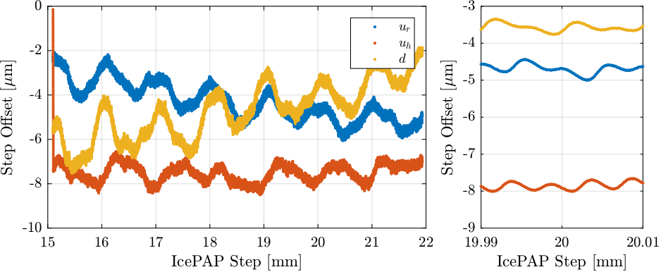
Figure 87: Computed LUT that will be used for further tests about the effect of the number of points taken in the trajectory
8.2. Trajectory with increment of \(1\,\mu m\)
A trajectory is loaded with 1000 points every millimeter of fast jack motion:
tdh.lut_constant_fj_vel(15.5, 21.5, pts_per_mm=1000, use_lut=True)
Several scans in mode B are performed and the results are shown in Figure
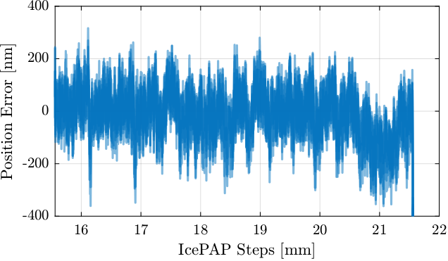
Figure 88: Measured position errors of the fast jacks
8.3. Trajectory with increment of \(0.4\,\mu m\)
A trajectory is loaded with 2500 points every millimeter of fast jack motion:
tdh.lut_constant_fj_vel(15.5, 21.5, pts_per_mm=2500, use_lut=True)
The obtained errors on fjur are shown in Figure 89.
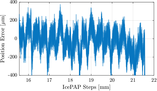
Figure 89: Measured position errors of the fast jacks
8.4. Spatial Errors - Comparison
The spatial periods of errors for the two trajectories are compared in Figure 90. Even though the trajectory with an increment of \(0.4\,\mu m\) was done after the trajectory with an increment of \(1\,\mu m\) (and therefore the errors in mode B should be higher), the errors for a period of \(5\,\mu m\) are reduced.
It should be further investigated whether using small increments for the trajectory could help reducing the \(5\,\mu m\) period errors.
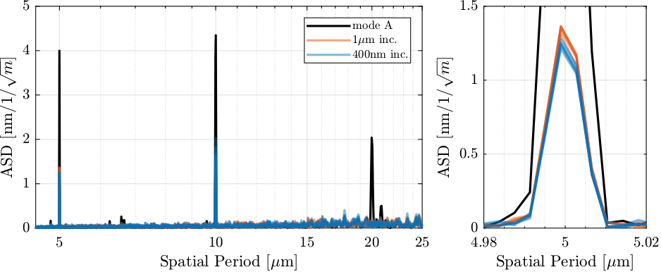
Figure 90: Spectral density of the fjur measured position errors for both trajectories. For the errors with a spatial periods of \(5\,\mu m\), taking smaller steps in the trajectory helps reducing the errors.
9. LUT for energy scans (XANES)
9.1. Velocities
%% Scan parameters
scan_name = {'P',  'S',  'Cl',  'Cd', 'Ca', 'Ti', 'V',  'Cr', 'Mn', 'Fe', 'Cu'}; % Element Name
start_ene = 1e3*[2.14, 2.45, 2.895, 3.52, 3.95, 4.94, 5.45, 5.98, 6.52, 7.1 , 8.98]; % [ev]
end_ene   = 1e3*[2.19, 2.55, 2.995, 3.65, 4.15, 5.1 , 5.57, 6.14, 6.75, 7.25, 9.12]; % [ev]
step_ene  = [0.25, 0.25, 0.3,   0.3,  0.4,  0.4,  0.5,  0.5,  0.5, 0.5, 0.5]; % Scan Steps [ev]

dwell_time_min = 0.01; % corresponds to max velocity [s]
dwell_time_max = 0.1;  % corresponds to min velocity [s]
dspacing = 3.13501196169967; % [Angstrom]
%% Scan objects
scans = {};
for i = 1:length(start_ene)
    scans{i}.name = scan_name{i};

    scans{i}.traj_ene   = start_ene(i):step_ene(i):end_ene(i); % [eV]
    scans{i}.traj_bragg = asin(12398.4./scans{i}.traj_ene/2/dspacing); % [rad]
    scans{i}.traj_fjs   = 0.030427 - (10.5e-3)./(2*cos(scans{i}.traj_bragg)); % [m]

    scans{i}.time_slow = dwell_time_max*0:1:length(scans{i}.traj_ene)-1; % [s]
    scans{i}.time_fast = dwell_time_min*0:1:length(scans{i}.traj_ene)-1; % [s]

    scans{i}.vel_fast_bragg = abs([scans{i}.traj_bragg(2:end) - scans{i}.traj_bragg(1:end-1), 0]/dwell_time_min); % [rad/s]
    scans{i}.vel_fast_fjs = abs([scans{i}.traj_fjs(2:end) - scans{i}.traj_fjs(1:end-1), 0]/dwell_time_min); % [m/s]
end
| Scan Name | FJ min [mm] | FJ max [mm] | FJ stroke [mm] | Max FJ vel [mm/s] |
|---|---|---|---|---|
| P | 16.696 | 18.212 | 1.516 | 0.936 |
| S | 21.535 | 22.112 | 0.577 | 0.169 |
| Cl | 23.239 | 23.437 | 0.198 | 0.065 |
| Cd | 24.081 | 24.181 | 0.1 | 0.025 |
| Ca | 24.362 | 24.456 | 0.093 | 0.021 |
| Ti | 24.698 | 24.731 | 0.033 | 0.009 |
| V | 24.793 | 24.811 | 0.018 | 0.008 |
| Cr | 24.864 | 24.882 | 0.017 | 0.006 |
| Mn | 24.918 | 24.936 | 0.019 | 0.004 |
| Fe | 24.961 | 24.97 | 0.009 | 0.003 |
| Cu | 25.045 | 25.049 | 0.004 | 0.002 |
| Scan Name | Bragg min [deg] | Bragg max [deg] | Bragg stroke [deg] | Max bragg vel [deg/s] |
|---|---|---|---|---|
| P | 64.545 | 67.521 | 2.976 | 0.719 |
| S | 50.846 | 53.814 | 2.968 | 0.355 |
| Cl | 41.32 | 43.082 | 1.762 | 0.247 |
| Cd | 32.804 | 34.178 | 1.374 | 0.147 |
| Ca | 28.456 | 30.04 | 1.584 | 0.149 |
| Ti | 22.813 | 23.596 | 0.783 | 0.09 |
| V | 20.794 | 21.274 | 0.48 | 0.091 |
| Cr | 18.787 | 19.309 | 0.522 | 0.075 |
| Mn | 17.035 | 17.655 | 0.62 | 0.062 |
| Fe | 15.828 | 16.171 | 0.343 | 0.052 |
| Cu | 12.522 | 12.721 | 0.198 | 0.032 |
Based on Table 6.
- To work without
mcoil, the maximum bragg stroke should be 16 degrees. Therefore, all the scans can be performed withoutmcoil.
Frequency of \(5\mu m\) errors:
| Scan Name | Max freq. [Hz] |
|---|---|
| P | 187.2 |
| S | 33.9 |
| Cl | 13.0 |
| Cd | 5.0 |
| Ca | 4.1 |
| Ti | 1.8 |
| V | 1.6 |
| Cr | 1.1 |
| Mn | 0.9 |
| Fe | 0.6 |
| Cu | 0.3 |
Estimation of maximum velocity such that the \(5\mu m\) errors are reduced by a factor 50 (i.e. the frequency of this \(5\mu m\) should be below 2Hz, see sensitivity function).
| Scan Name | Min time [s] - 2Hz | Min time [s] - 10Hz |
|---|---|---|
| P | 0.9358 | 0.1872 |
| S | 0.1695 | 0.0339 |
| Cl | 0.0651 | 0.013 |
| Cd | 0.0249 | 0.005 |
| Ca | 0.0205 | 0.0041 |
| Ti | 0.0088 | 0.0018 |
| V | 0.0078 | 0.0016 |
| Cr | 0.0057 | 0.0011 |
| Mn | 0.0043 | 0.0009 |
| Fe | 0.0032 | 0.0006 |
| Cu | 0.0015 | 0.0003 |
9.2. test
%% Scan parameters
start_ene = 1e3*2.21; % [ev]
end_ene   = 1e3*2.23; % [ev]
step_ene  = 0.2;

dwell_time_min = 0.01; % corresponds to max velocity [s]
dwell_time_max = 0.1;  % corresponds to min velocity [s]
dspacing = 3.13501196169967; % [Angstrom]
%% Scan objects
traj_ene   = start_ene:step_ene:end_ene; % [eV]
traj_bragg = asin(12398.4./traj_ene/2/dspacing); % [rad]
traj_fjs   = 0.030427 - (10.5e-3)./(2*cos(traj_bragg)); % [m]

time_slow = dwell_time_max*0:1:length(traj_ene)-1; % [s]
time_fast = dwell_time_min*0:1:length(traj_ene)-1; % [s]

vel_fast_bragg = abs([traj_bragg(2:end) - traj_bragg(1:end-1), 0]/dwell_time_min); % [rad/s]
vel_fast_fjs = abs([traj_fjs(2:end) - traj_fjs(1:end-1), 0]/dwell_time_min); % [m/s]
figure; plot(time_fast, 1e3*vel_fast_fjs)
| Scan Name | FJ min [mm] | FJ max [mm] | FJ stroke [mm] | Max FJ vel [mm/s] |
|---|---|---|---|---|
| P | 16.696 | 18.212 | 1.516 | 0.936 |
| S | 21.535 | 22.112 | 0.577 | 0.169 |
| Cl | 23.239 | 23.437 | 0.198 | 0.065 |
| Cd | 24.081 | 24.181 | 0.1 | 0.025 |
| Ca | 24.362 | 24.456 | 0.093 | 0.021 |
| Ti | 24.698 | 24.731 | 0.033 | 0.009 |
| V | 24.793 | 24.811 | 0.018 | 0.008 |
| Cr | 24.864 | 24.882 | 0.017 | 0.006 |
| Mn | 24.918 | 24.936 | 0.019 | 0.004 |
| Fe | 24.961 | 24.97 | 0.009 | 0.003 |
| Cu | 25.045 | 25.049 | 0.004 | 0.002 |
| Scan Name | Bragg min [deg] | Bragg max [deg] | Bragg stroke [deg] | Max bragg vel [deg/s] |
|---|---|---|---|---|
| P | 64.545 | 67.521 | 2.976 | 0.719 |
| S | 50.846 | 53.814 | 2.968 | 0.355 |
| Cl | 41.32 | 43.082 | 1.762 | 0.247 |
| Cd | 32.804 | 34.178 | 1.374 | 0.147 |
| Ca | 28.456 | 30.04 | 1.584 | 0.149 |
| Ti | 22.813 | 23.596 | 0.783 | 0.09 |
| V | 20.794 | 21.274 | 0.48 | 0.091 |
| Cr | 18.787 | 19.309 | 0.522 | 0.075 |
| Mn | 17.035 | 17.655 | 0.62 | 0.062 |
| Fe | 15.828 | 16.171 | 0.343 | 0.052 |
| Cu | 12.522 | 12.721 | 0.198 | 0.032 |
Based on Table 6.
- To work without
mcoil, the maximum bragg stroke should be 16 degrees. Therefore, all the scans can be performed withoutmcoil.
Frequency of \(5\mu m\) errors:
| Scan Name | Max freq. [Hz] |
|---|---|
| P | 187.2 |
| S | 33.9 |
| Cl | 13.0 |
| Cd | 5.0 |
| Ca | 4.1 |
| Ti | 1.8 |
| V | 1.6 |
| Cr | 1.1 |
| Mn | 0.9 |
| Fe | 0.6 |
| Cu | 0.3 |
Estimation of maximum velocity such that the \(5\mu m\) errors are reduced by a factor 50 (i.e. the frequency of this \(5\mu m\) should be below 2Hz, see sensitivity function).
| Scan Name | Min time [s] - 2Hz | Min time [s] - 10Hz |
|---|---|---|
| P | 0.9358 | 0.1872 |
| S | 0.1695 | 0.0339 |
| Cl | 0.0651 | 0.013 |
| Cd | 0.0249 | 0.005 |
| Ca | 0.0205 | 0.0041 |
| Ti | 0.0088 | 0.0018 |
| V | 0.0078 | 0.0016 |
| Cr | 0.0057 | 0.0011 |
| Mn | 0.0043 | 0.0009 |
| Fe | 0.0032 | 0.0006 |
| Cu | 0.0015 | 0.0003 |
10. Merge LUT
10.1. Merge LUT
lut_10_15 = importdata("LUT_220202_10_to_15_1.dat");
lut_15_45 = importdata("LUT_220202_15_to_45_1.dat");
lut_45_75 = importdata("LUT_220202_45_to_75_1.dat");
% [ur, uh, d]
a = [25.07, 25.09, 24.92];
b = [23.06, 23.1 , 22.93];
cond_45_75 = lut_45_75(:,1) < b(1);
cond_15_45 = lut_15_45(:,1) > b(1) & lut_15_45(:,1) < a(1);
cond_10_15 = lut_10_15(:,1) > a(1);

cond_45_75_ur = lut_45_75(:,1) < b(1);
cond_15_45_ur = lut_15_45(:,1) > b(1) & lut_15_45(:,1) < a(1);
cond_10_15_ur = lut_10_15(:,1) > a(1);

cond_45_75_uh = lut_45_75(:,1) < b(2);
cond_15_45_uh = lut_15_45(:,1) > b(2) & lut_15_45(:,1) < a(2);
cond_10_15_uh = lut_10_15(:,1) > a(2);

cond_45_75_d  = lut_45_75(:,1) < b(3);
cond_15_45_d  = lut_15_45(:,1) > b(3) & lut_15_45(:,1) < a(3);
cond_10_15_d  = lut_10_15(:,1) > a(3);
lut_ind = [lut_45_75(cond_45_75, 1);
           lut_15_45(cond_15_45, 1);
           lut_10_15(cond_10_15, 1)];

lut_ur = [lut_45_75(cond_45_75_ur, 2);
          lut_15_45(cond_15_45_ur, 2);
          lut_10_15(cond_10_15_ur, 2)];

lut_uh = [lut_45_75(cond_45_75_uh, 3);
          lut_15_45(cond_15_45_uh, 3);
          lut_10_15(cond_10_15_uh, 3)];

lut_d  = [lut_45_75(cond_45_75_d, 4);
          lut_15_45(cond_15_45_d, 4);
          lut_10_15(cond_10_15_d, 4)];
lut = [lut_ind, lut_ur, lut_uh, lut_d];
%% Save lut as a .dat file
formatSpec = '%.18e %.18e %.18e %.18e\n';

fileID = fopen("LUT_220202_10_to_75_1_merged.mat", 'w');
fprintf(fileID, formatSpec, lut');
fclose(fileID);