ESRF Double Crystal Monochromator - Metrology
Table of Contents
This report is also available as a pdf.
In this document, the metrology system is studied. First, in Section 1 the goal of the metrology system is stated and the proposed concept is described.
How the relative crystal pose is affecting the pose of the output beam is studied in Section 2.
In order to increase the accuracy of the metrology system, two problems are to be dealt with:
- The deformation of the metrology frame under the action of gravity (Section 4)
- The periodic non-linearity of the interferometers (Section 5)
1. Metrology Concept
The goal of the metrology system is to measure the distance and default of parallelism between the first and second crystals.
Only 3 degrees of freedom are of interest:
- \(d_z\)
- \(r_y\)
- \(r_x\)
1.1. Sensor Topology
In order to measure the relative pose of the two crystals, instead of performing a direct measurement which is complicated, the pose of the two crystals are measured from a metrology frame. Three interferometers are used to measured the 3dof of interest for each crystals. Three additional interferometers are used to measured the relative motion of the metrology frame.
In total, there are 15 interferometers represented in Figure 1. The measurements are summarized in Table 2.
| Notation | Meaning |
|---|---|
d |
“Downstream”: Positive X |
u |
“Upstream”: Negative X |
h |
“Hall”: Positive Y |
r |
“Ring”: Negative Y |
f |
“Frame” |
1 |
“First Crystals” |
2 |
“Second Crystals” |
| Number | Measurement | Description |
|---|---|---|
| 1 | \(z_{1r,u}\) | First “Ring” Crystal, “upstream” |
| 2 | \(z_{1r,c}\) | First “Ring” Crystal, “center” |
| 3 | \(z_{1r,d}\) | First “Ring” Crystal, “downstream” |
| 4 | \(z_{1h,u}\) | First “Hall” Crystal, “upstream” |
| 5 | \(z_{1h,c}\) | First “Hall” Crystal, “center” |
| 6 | \(z_{1h,d}\) | First “Hall” Crystal, “downstream” |
| 7 | \(z_{2h,u}\) | Second “Hall” Crystal, “upstream” |
| 8 | \(z_{2h,c}\) | Second “Hall” Crystal, “center” |
| 9 | \(z_{2h,d}\) | Second “Hall” Crystal, “downstream” |
| 10 | \(z_{2r,u}\) | Second “Ring” Crystal, “upstream” |
| 11 | \(z_{2r,c}\) | Second “Ring” Crystal, “center” |
| 12 | \(z_{2r,d}\) | Second “Ring” Crystal, “downstream” |
| 13 | \(z_{mf,u}\) | Metrology Frame, “upstream” |
| 14 | \(z_{mf,dr}\) | Metrology Frame, “downstream-ring” |
| 15 | \(z_{mf,dh}\) | Metrology Frame, “downstream-hall” |
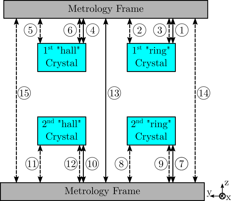
Figure 1: Schematic of the Metrology System
1.2. Computation of the relative pose between first and second crystals
To understand how the relative pose between the crystals is computed from the interferometer signals, have a look at this repository (https://gitlab.esrf.fr/dehaeze/dcm-kinematics).
Basically, Jacobian matrices are derived from the geometry and are used to convert the 15 interferometer signals to the relative pose of the primary and secondary crystals \([d_{h,z},\ r_{h,y},\ r_{h,x}]\) or \([d_{r,z},\ r_{r,y},\ r_{r,x}]\).
The sign conventions for the relative crystal pose are:
- An increase of \(d_{h,z}\) means the two crystals are further apart
- An increase of \(r_{h,}\) means that the second crystals experiences a rotation around \(y\) with respect to the primary crystal
- An increase of \(r_{h,x}\) means that the second crystals experiences a rotation around \(x\) with respect to the primary crystal
The relative pose can be expressed as a function of the interferometers using the Jacobian matrices for the “hall” crystals:
\begin{equation} \boxed{ \begin{bmatrix} d_{h,z} \\ r_{h,y} \\ r_{h,x} \end{bmatrix} = \bm{J}_{2h,s}^{-1} \begin{bmatrix} z_{2h,u} \\ z_{2h,c} \\ z_{2h,d} \end{bmatrix} - \bm{J}_{1h,s}^{-1} \begin{bmatrix} z_{1h,u} \\ z_{1h,c} \\ z_{1h,d} \end{bmatrix} - \bm{J}_{mf,s}^{-1} \begin{bmatrix} z_{mf,u} \\ z_{mf,dh} \\ z_{mf,dr} \end{bmatrix} } \end{equation}As well as for the “ring” crystals:
\begin{equation} \boxed{ \begin{bmatrix} d_{r,z} \\ r_{r,y} \\ r_{r,x} \end{bmatrix} = \bm{J}_{2r,s}^{-1} \begin{bmatrix} z_{2r,u} \\ z_{2r,c} \\ z_{2r,d} \end{bmatrix} - \bm{J}_{1r,s}^{-1} \begin{bmatrix} z_{1r,u} \\ z_{1r,c} \\ z_{1r,d} \end{bmatrix} - \bm{J}_{mf,s}^{-1} \begin{bmatrix} z_{mf,u} \\ z_{mf,dr} \\ z_{mf,dr} \end{bmatrix} } \end{equation}
Values of the matrices can be found in the document describing the kinematics of the DCM (see https://gitlab.esrf.fr/dehaeze/dcm-kinematics).
2. Relation Between Crystal position and X-ray measured displacement
In this section, the impact of an error in the relative pose between the first and second crystals on the output X-ray beam is studied.
This is very important in order to:
- link a measurement of the x-ray beam position to a default in the crystal position
- understand which pose default will have large impact on the output beam position/orientation
- calibrate the deformations of the metrology frame using an external metrology measuring the x-ray beam position/orientation
In order to simplify the problem, the first crystal is supposed to be fixed (i.e. ideally positioned), and only the motion of the second crystal is studied.
In order to easily study that, “ray tracing” techniques are used.
2.1. Definition of frame
| Position | Orientation | |
|---|---|---|
| input beam | x1,y1,z1 |
s1 |
| primary mirror | xp,yp,zp |
np |
| reflected beam | x2,y2,z2 |
s2 |
| secondary mirror | xs,ys,zz |
ns |
| output beam | x3,y3,z3 |
s3 |
| Dectector | xd,yd,zd |
nd |
[ ]Add schematic
Notations for the pose of the output beam: d_b_y, d_b_z, r_b_y, r_b_z.
\(d_{b,y}, d_{b,z}, r_{b,y}, r_{b,z}\)
The xy position of the beam is taken in the \(x=0\) plane.
2.2. Effect of an error in crystal’s distance
In Figure 2 is shown the light path for three bragg angles (5, 55 and 85 degrees) when there is an error in the dz position of 1mm.
Visually, it is clear that this induce a z offset of the output beam.

Figure 2: Visual Effect of an error in dz (1mm). Side view.
The motion of the output beam is displayed as a function of the Bragg angle in Figure 3.
It is clear that an error in the distance dz between the crystals only induce a z offset of the output beam.
This offset decreases with the Bragg angle.
This is indeed equal to:
\begin{equation} \boxed{d_{b,z} = 2 d_z \cos \theta} \end{equation}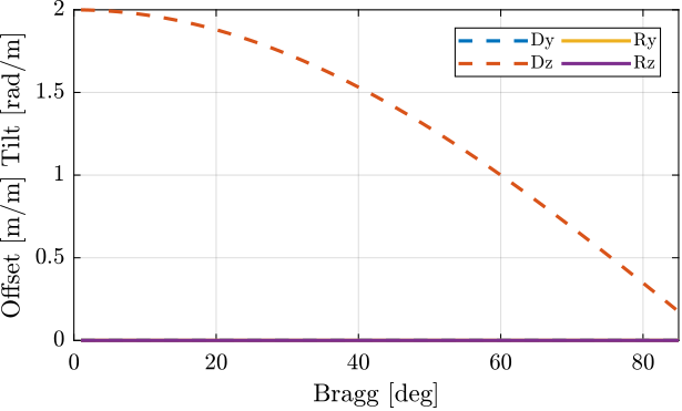
Figure 3: Motion of the output beam with dZ error
2.3. Effect of an error in crystal’s x parallelism
The effect of an error in rx crystal parallelism on the output beam is visually shown in Figure 4 for three bragg angles (5, 55 and 85 degrees).
The error is set to one degree, and the top view is shown.
It is clear that the output beam experiences some rotation around a vertical axis.
The amount of rotation depends on the bragg angle.
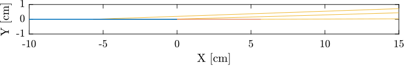
Figure 4: Visual Effect of an error in drx (1 degree). Top View.
The effect of drx as a function of the Bragg angle on the output beam pose is computed and shown in Figure 5.
It induces a rotation of the output beam in the z direction that depends on the Bragg Angle.
It is starting at zero for small bragg angles, and it increases with the bragg angle up to 2 times drx.
This is indeed equal to:
If also induces a small \(y\) shift of the beam. This shift is due to the fact that the rotation point (around which the second crystal is moved) is changing as a function of bragg. We can note that the \(y\) shift is equal to zero for a bragg angle of 45 degrees, at which point the center of rotation of the second crystal is at \(x = 0\);
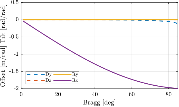
Figure 5: Motion of the output beam with drx error
2.4. Effect of an error in crystal’s y parallelism
The effect of an error in ry crystal parallelism on the output beam is visually shown in Figure 6 for three bragg angles (5, 55 and 85 degrees).
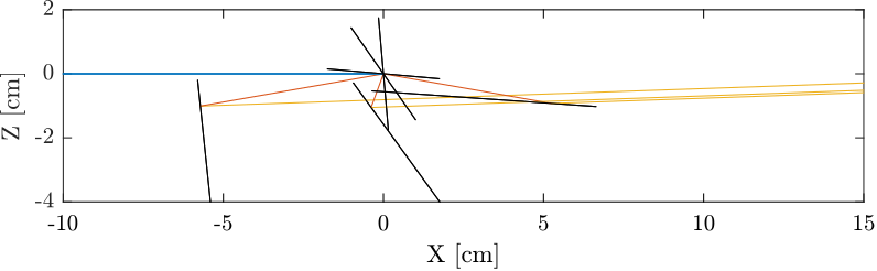
Figure 6: Visual Effect of an error in dry (1 degree). Side view.
The effect of dry as a function of the Bragg angle on the output beam pose is computed and shown in Figure 7.
It is clear that this induces a rotation of the output beam in the y direction equals to 2 times dry:
It also induces a small vertical motion of the beam (at the \(x=0\) location) which is simply due to the fact that the \(x\) coordinate of the impact point on the second crystal changes with the Bragg angle.
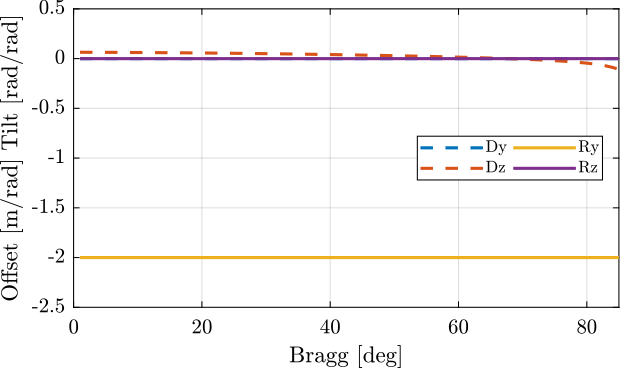
Figure 7: Motion of the output beam with dry error
2.5. Summary
Effects of crystal’s pose errors on the output beam are summarized in Table 3. Note that the three pose errors are well decoupled regarding their effects on the output beam. Also note that the effect of an error in crystal’s distance does not depend on the Bragg angle.
| Beam Motion | Crystal \(d_z\) | Crystal \(r_x\) | Crystal \(r_y\) |
|---|---|---|---|
| \(d_{b,y}\) | 0 | \(\approx 0\) | 0 |
| \(d_{b,z}\) | \(\boxed{d_{z} 2 \cos(\theta)}\) | 0 | \(\approx 0\) |
| \(r_{b,y}\) | 0 | 0 | \(\boxed{2 r_{y}}\) |
| \(r_{b,z}\) | 0 | \(\boxed{- r_x 2 \sin(\theta)}\) | 0 |
2.6. “Channel cut” Scan
A “channel cut” scan is a Bragg scan where the distance between the crystals is fixed.
This is visually shown in Figure 8 where it is clear that the output beam experiences some vertical motion.
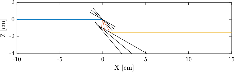
Figure 8: Visual Effect of a channel cut scan
The \(z\) offset of the beam for several channel cut scans are shown in Figure 9.
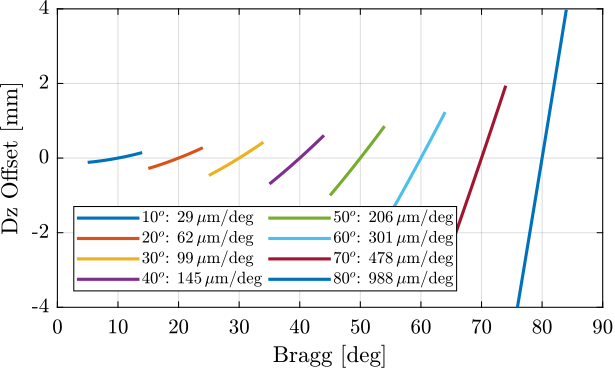
Figure 9: Z motion of the beam during “channel cut” scans
3. Determining relative pose between the crystals using the X-ray
As Interferometers are only measuring relative displacement, it is mandatory to initialize them correctly.
They should be initialize in such a way that:
- \(r_x = 0\) and \(r_y = 0\) when the two crystallographic planes are parallel
- measured \(d_z\) is equal to the distance between the crystallographic planes
In order to do that, an external metrology using the x-ray is used.
3.1. Determine the \(y\) parallelism - “Rocking Curve”
3.2. Determine the \(x\) parallelism - Bragg Scan
3.3. Determine the \(z\) distance - Bragg Scan
3.4. Use Channel cut scan to determine crystal dry parallelism
Now, let’s suppose we want to determine the dry angle between the crystals.
dry = 1e-6; % [rad]
The error is
\begin{equation} \boxed{d_{b,z} = -2 d_z \cos()} \end{equation}3.5. Effect of an error on Bragg angle
4. Deformations of the Metrology Frame
The transformation matrices are valid only if the metrology frames are solid bodies.
The metrology frame itself is experiencing some deformations due to the gravity. When the bragg axis is scanned, the effect of gravity on the metrology frame is changing and this introduce some measurement errors.
This can be calibrated.
4.1. Measurement Setup
Two beam viewers:
- one close to the DCM to measure position of the beam
- one far away to the DCM to measure orientation of the beam
For each Bragg angle, the Fast Jacks are actuated to that the beam is at the center of the beam viewer. Then, then position of the crystals as measured by the interferometers is recorded. This position is the wanted position for a given Bragg angle.
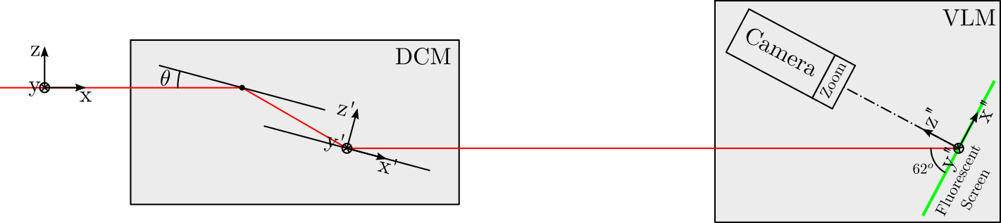
Figure 10: Schematic of the setup
Detector:
https://www.baslerweb.com/en/products/cameras/area-scan-cameras/ace/aca1920-40gc/
Pixel size depends on the magnification used (1x, 6x, 12x).
Pixel size of camera is 5.86 um x 5.86 um. With typical magnification of 6x, pixel size is ~1.44um x 1.44um
Frame rate is: 42 fps
4.2. Simulations
The deformations of the metrology frame and therefore the expected interferometric measurements can be computed as a function of the Bragg angle. This may be done using FE software.
4.3. Comparison
4.4. Test
aa = importdata("correctInterf-vlm-220201.dat");
figure;
plot(aa.data(:,1), aa.data(:,24))
4.5. Measured frame deformation
data = table2array(readtable('itf_polynom.csv','NumHeaderLines',1));
th = pi/180*data(:,1); % [rad]
fj = 0.030427 - 10.51e-3./(2*cos(th)); % [m]
rx2 = 1e-9*data(:,2); % [rad]
ry2 = 1e-9*data(:,3); % [rad]
rx1 = 1e-9*data(:,4); % [rad]
ry1 = 1e-9*data(:,5); % [rad]
figure;
hold on;
plot(180/pi*th, 1e6*detrend(-rx2, 1), '.')
% plot(180/pi*th, detrend(ry2, 1))
% plot(180/pi*th, detrend(rx1, 1))
% plot(180/pi*th, detrend(ry1, 1))
hold off;
xlabel('Bragg Angle [deg]');
ylabel('Measured $R_x$ [$\mu$rad]')
xlim([10, 75]);
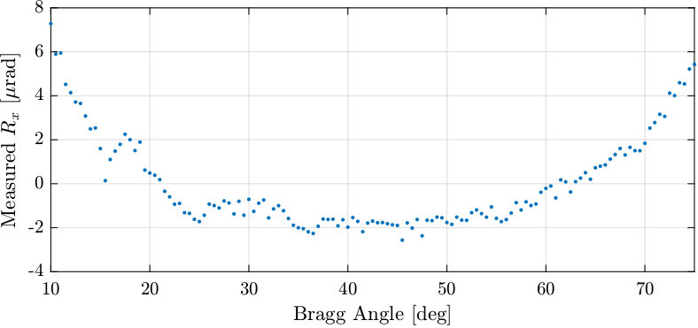
Figure 11: description
Strange that there is correlation between Rx and Ry.
figure;
hold on;
plot(108/pi*th, 1e9*detrend(rx1, 0), '-', 'DisplayName', '$Rx_1$')
plot(108/pi*th, 1e9*detrend(ry1, 0), '-', 'DisplayName', '$Ry_1$')
hold off;
xlabel('Bragg Angle [deg]'); ylabel('Angle Offset [nrad]');
legend()
figure;
hold on;
plot(1e3*fj, detrend(rx2, 1), 'DisplayName', '$Rx_1$')
plot(1e3*fj, detrend(ry2, 1), 'DisplayName', '$Ry_1$')
hold off;
xlabel('Fast Jack Displacement [mm]'); ylabel('Angle Offset [nrad]');
legend()
%% Compute best polynomial fit
f_rx2 = fit(180/pi*th, 1e9*rx2, 'poly4');
f_ry2 = fit(180/pi*th, 1e9*ry2, 'poly4');
f_rx1 = fit(180/pi*th, 1e9*rx1, 'poly4');
f_ry1 = fit(180/pi*th, 1e9*ry1, 'poly4');
figure;
hold on;
plot(180/pi*th, f_rx2(180/pi*th))
plot(180/pi*th, f_ry2(180/pi*th))
plot(180/pi*th, f_rx1(180/pi*th))
plot(180/pi*th, f_ry1(180/pi*th))
hold off;
figure;
hold on;
plot(th, f_rx2(th) - rx2)
plot(th, f_ry2(th) - ry2)
plot(th, f_rx1(th) - rx1)
plot(th, f_ry1(th) - ry1)
hold off;
figure;
hold on;
plot(th, f(th))
plot(th, rx2, '.')
4.6. Test
filename = "/home/thomas/mnt/data_id21/22Jan/blc13550/id21/test_xtal1_interf/test_xtal1_interf_0001/test_xtal1_interf_0001.h5";
data = struct();

data.xtal1_111_u = double(h5read(filename, '/7.1/instrument/FPGA1_SSIM4/data'));
data.xtal1_111_m = double(h5read(filename, '/7.1/instrument/FPGA1_SSIM5/data'));
data.xtal1_111_d = double(h5read(filename, '/7.1/instrument/FPGA1_SSIM6/data'));
data.mframe_u = double(h5read(filename, '/7.1/instrument/FPGA2_SSIM3/data'));
data.mframe_dh = double(h5read(filename, '/7.1/instrument/FPGA2_SSIM4/data'));
data.mframe_dr = double(h5read(filename, '/7.1/instrument/FPGA2_SSIM5/data'));
data.bragg = (pi/180)*double(h5read(filename, '/7.1/instrument/FPGA2_SSIM6/data'));
data.fj_pos = 0.030427 - 10.5e-3./(2*cos(data.bragg));
data.time  = double(h5read(filename, '/7.1/instrument/time/data'));
data.rx    = 1e-9*double(h5read(filename, '/7.1/instrument/xtal1_111_rx/data'));
data.ry    = 1e-9*double(h5read(filename, '/7.1/instrument/xtal1_111_ry/data'));
data.z     = 1e-9*double(h5read(filename, '/7.1/instrument/xtal1_111_z/data'));
data.drx   = 1e-9*double(h5read(filename, '/7.1/instrument/xtal_111_drx_filter/data'));
data.dry   = 1e-9*double(h5read(filename, '/7.1/instrument/xtal_111_dry_filter/data'));
data.dz    = 1e-9*double(h5read(filename, '/7.1/instrument/xtal_111_dz_filter/data'));
data.xtal2_111_u = double(h5read(filename, '/7.1/instrument/FPGA1_SSIM10/data'))+10.5e6./(2*cos(data.bragg));
data.xtal2_111_m = double(h5read(filename, '/7.1/instrument/FPGA2_SSIM1/data'))+10.5e6./(2*cos(data.bragg));
data.xtal2_111_d = double(h5read(filename, '/7.1/instrument/FPGA2_SSIM2/data'))+10.5e6./(2*cos(data.bragg));
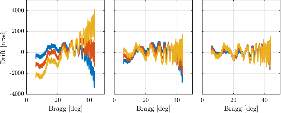
Figure 12: Drifts of the second crystal as a function of Bragg Angle
figure;
hold on;
plot(108/pi*data.bragg, data.drx)
plot(108/pi*data.bragg, data.dry)
hold off;
4.7. Repeatability of frame deformation
filename = "/home/thomas/mnt/data_id21/22Jan/blc13550/id21/test_xtal1_interf/test_xtal1_interf_0001/test_xtal1_interf_0001.h5";
data_1 = struct();
data_1.time  = double(h5read(filename, '/7.1/instrument/time/data'));
data_1.bragg = (pi/180)*double(h5read(filename, '/7.1/instrument/FPGA2_SSIM6/data'));
data_1.fj_pos = 0.030427 - 10.5e-3./(2*cos(data_1.bragg));
data_1.xtal1_111_u = double(h5read(filename, '/7.1/instrument/FPGA1_SSIM4/data'));
data_1.xtal1_111_m = double(h5read(filename, '/7.1/instrument/FPGA1_SSIM5/data'));
data_1.xtal1_111_d = double(h5read(filename, '/7.1/instrument/FPGA1_SSIM6/data'));
data_1.xtal2_111_u = double(h5read(filename, '/7.1/instrument/FPGA1_SSIM10/data'))+10.5e6./(2*cos(data_1.bragg));
data_1.xtal2_111_m = double(h5read(filename, '/7.1/instrument/FPGA2_SSIM1/data'))+10.5e6./(2*cos(data_1.bragg));
data_1.xtal2_111_d = double(h5read(filename, '/7.1/instrument/FPGA2_SSIM2/data'))+10.5e6./(2*cos(data_1.bragg));
data_1.mframe_u = double(h5read(filename, '/7.1/instrument/FPGA2_SSIM3/data'));
data_1.mframe_dh = double(h5read(filename, '/7.1/instrument/FPGA2_SSIM4/data'));
data_1.mframe_dr = double(h5read(filename, '/7.1/instrument/FPGA2_SSIM5/data'));
data_1.drx   = 1e-9*double(h5read(filename, '/7.1/instrument/xtal_111_drx_filter/data'));
data_1.dry   = 1e-9*double(h5read(filename, '/7.1/instrument/xtal_111_dry_filter/data'));
data_1.dz    = 1e-9*double(h5read(filename, '/7.1/instrument/xtal_111_dz_filter/data'));
data_2 = struct();
data_2.time  = double(h5read(filename, '/6.1/instrument/time/data'));
data_2.bragg = (pi/180)*double(h5read(filename, '/6.1/instrument/FPGA2_SSIM6/data'));
data_2.fj_pos = 0.030427 - 10.5e-3./(2*cos(data_2.bragg));
data_2.xtal1_111_u = double(h5read(filename, '/6.1/instrument/FPGA1_SSIM4/data'));
data_2.xtal1_111_m = double(h5read(filename, '/6.1/instrument/FPGA1_SSIM5/data'));
data_2.xtal1_111_d = double(h5read(filename, '/6.1/instrument/FPGA1_SSIM6/data'));
data_2.xtal2_111_u = double(h5read(filename, '/6.1/instrument/FPGA1_SSIM10/data'))+10.5e6./(2*cos(data_2.bragg));
data_2.xtal2_111_m = double(h5read(filename, '/6.1/instrument/FPGA2_SSIM1/data'))+10.5e6./(2*cos(data_2.bragg));
data_2.xtal2_111_d = double(h5read(filename, '/6.1/instrument/FPGA2_SSIM2/data'))+10.5e6./(2*cos(data_2.bragg));
data_2.mframe_u = double(h5read(filename, '/6.1/instrument/FPGA2_SSIM3/data'));
data_2.mframe_dh = double(h5read(filename, '/6.1/instrument/FPGA2_SSIM4/data'));
data_2.mframe_dr = double(h5read(filename, '/6.1/instrument/FPGA2_SSIM5/data'));
data_2.drx   = 1e-9*double(h5read(filename, '/6.1/instrument/xtal_111_drx_filter/data'));
data_2.dry   = 1e-9*double(h5read(filename, '/6.1/instrument/xtal_111_dry_filter/data'));
data_2.dz    = 1e-9*double(h5read(filename, '/6.1/instrument/xtal_111_dz_filter/data'));
5. Attocube - Periodic Non-Linearity
Interferometers have some periodic nonlinearity (NO_ITEM_DATA:thurner15_fiber_based_distan_sensin_inter). The period is a fraction of the wavelength (usually \(\lambda/2\)) and can be due to polarization mixing, non perfect alignment of the optical components and unwanted reflected beams (See NO_ITEM_DATA:ducourtieux18_towar_high_precis_posit_contr, NO_ITEM_DATA:thurner15_fiber_based_distan_sensin_inter). The amplitude of the nonlinearity can vary from a fraction of a nanometer to tens of nanometers.
In the DCM case, when using Attocube interferometers, the period non-linearity are in the order of several nanometers with a period of \(765\,nm\). This is inducing some positioning errors which are too high.
In order to overcome this issue, the periodic non-linearity of the interferometers have to be calibrated. To do so, a displacement is imposed and measured both by the interferometers and by another metrology system which does not have this nonlinearity. By comparing the two measured displacements, the nonlinearity can be calibration. This process is performed over several periods in order to characterize the error over the full stroke.
5.1. Measurement Setup
The metrology that will be compared with the interferometers are the strain gauges incorporated in the PI piezoelectric stacks.
It is here supposed that the measured displacement by the strain gauges are converted to the displacement at the interferometer locations. It is also supposed that we are at a certain Bragg angle, and that the stepper motors are not moving: only the piezoelectric actuators are used.
Note that the strain gauges are measuring the relative displacement of the piezoelectric stacks while the interferometers are measuring the relative motion between the second crystals and the metrology frame.
Only the interferometers measuring the second crystal motion can be calibrated here.
As any deformations of the metrology frame of deformation of the crystal’s support can degrade the quality of the calibration, it is better to perform this calibration without any bragg angle motion.
The setup is schematically with the block diagram in Figure 13.
The signals are:
- \(u\): Reference Signal sent to the PI controller (position where we wish to three stacks to be). The PI controller takes care or controlling to position as measured by the strain gauges such that it is close to the reference position.
- \(d\): Disturbances affecting the position of the crystals
- \(y\): Displacement of the crystal as measured by one interferometer
- \(y_g\): Measurement of the motion in the frame of the interferometer by the strain gauge with some noise \(n_g\)
- \(y_a\): Measurement of the crystal motion by the interferometer with some noise \(n_a\)
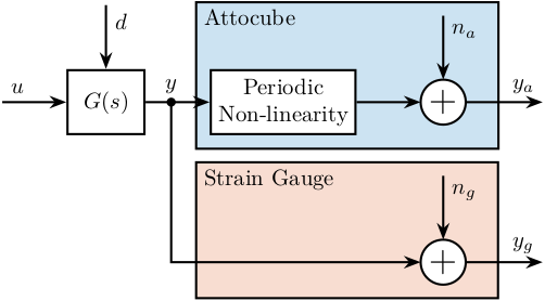
Figure 13: Block Diagram schematic of the setup used to measure the periodic non-linearity of the Attocube
The problem is to estimate the periodic non-linearity of the Attocube from the imperfect measurements \(y_a\) and \(y_g\).
5.2. Choice of the reference signal
The main specifications for the reference signal are;
- sweep several periods (i.e. several micrometers)
- stay in the linear region of the strain gauge
- no excitation of mechanical modes (i.e. the frequency content of the signal should be at low frequency)
- no phase shift due to limited bandwidth of both the interferometers and the strain gauge
- the full process should be quite fast
The travel range of the piezoelectric stacks is 15 micrometers, the resolution of the strain gauges is 0.3nm and the maximum non-linearity is 0.15%. If one non-linear period is swept (765nm), the maximum estimation error of the strain gauge is around 1nm.
Based on the above discussion, one suitable excitation signal is a sinusoidal sweep with a frequency of 10Hz.
5.3. Repeatability of the non-linearity
Instead of calibrating the non-linear errors of the interferometers over the full fast jack stroke (25mm), one can only calibrate the errors of one period.
For that, we need to make sure that the errors are repeatable from one period to the other and also the period should be very precisely estimated (i.e. the wavelength of the laser).
Also, the laser wavelength should be very stable (specified at 50ppb).
One way to precisely estimate the laser wavelength is to estimate the non linear errors of the interferometer at an initial position, and then to estimate the non linear errors at a large offset, say 10mm.
5.4. Simulation
Suppose we have a first approximation of the non-linear period.
period_est = 765e-9; % Estimated period [m]
And suppose the real period of the non-linear errors is a little bit above (by 0.02nm):
period_err = 0.02e-9; % Error on the period estimation [m]
period_nl = period_est + period_err; % Period of the non-linear errors [m]
The non-linear errors are first estimated at the beginning of the stroke (Figure 14).
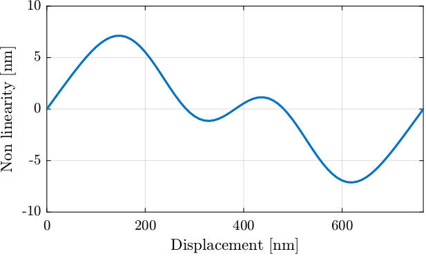
Figure 14: Estimation of the non-linear errors at the beginning of the stroke
From this only measurement, it is not possible to estimate with great accuracy the period of the error. To do so, the same measurement is performed with a stroke of several millimeters (Figure 15).
It can be seen that there is an offset between the estimated and the measured errors. This is due to a mismatch between the estimated period and the true period of the error.
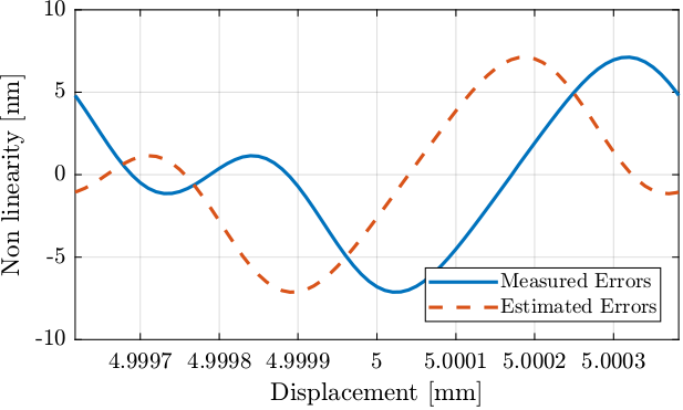
Figure 15: Estimated non-linear errors at a latter position
Suppose the non-linear error is characterized by a periodic function \(\mathcal{E}\), to simplify let’s take a sinusoidal function (this can be generalized by taking the fourier transform of the function):
\begin{equation} \mathcal{E}(x) = \sin\left(\frac{x}{\lambda}\right) \end{equation}with \(x\) the displacement and \(\lambda\) the period of the error.
The measured error at \(x_0\) is then:
\begin{equation} \mathcal{E}_m(x_0) = \sin\left( \frac{x_0}{\lambda} \right) \end{equation}And the estimated one is:
\begin{equation} \mathcal{E}_e(x_0) = \sin \left( \frac{x_0}{\lambda_{\text{est}}} \right) \end{equation}with \(\lambda_{\text{est}}\) the estimated error’s period.
From Figure 15, we can see that there is an offset between the two curves. Let’s call this offset \(\epsilon_x\), we then have:
\begin{equation} \mathcal{E}_m(x_0) = \mathcal{E}_e(x_0 + \epsilon_x) \end{equation}Which gives us:
\begin{equation} \sin\left( \frac{x_0}{\lambda} \right) = \sin \left( \frac{x_0 + \epsilon_x}{\lambda_{\text{est}}} \right) \end{equation}Finally:
\begin{equation} \boxed{\lambda = \lambda_{\text{est}} \frac{x_0}{x_0 + \epsilon_x}} \end{equation}The estimated delay is computed:
%% Estimation of the offset between the estimated and measured errors
i_period = stroke > 5e-3-period_nl/2 & stroke < 5e-3+period_nl/2;
epsilon_x = finddelay(nl_errors(i_period), est_errors(i_period)) % [m]
Estimated delay x0 is -120 [nm]
And the period \(\lambda\) can be estimated:
%% Computation of the period [m]
period_fin = period_est * (5e-3)/(5e-3 + d_offset); % Estimated period after measurement [m]
The estimated period is 765.020 [nm]
And the results confirms that this method is working on paper.
When doing this computation, we suppose that there are at most one half period of offset between the estimated and the measured non-linear (to not have any ambiguity whether the estimated period is too large or too small). Mathematically this means that the displacement \(x_0\) should be smaller than:
\begin{equation} x_0 < \frac{1}{2} \cdot \lambda \cdot \frac{\lambda}{\epsilon_\lambda} \end{equation}With \(\epsilon_\lambda\) the absolute estimation error of the period in meters.
For instance, if we estimate the error on the period to be less than 0.1nm, the maximum displacement is:
%% Estimated maximum stroke [m]
max_x0 = 0.5 * 765e-9 * (765e-9)/(0.1e-9);
The maximum stroke is 2.9 [mm]
5.5. Measurements
We have some constrains on the way the motion is imposed and measured:
- We want the frequency content of the imposed motion to be at low frequency in order not to induce vibrations of the structure. We have to make sure the forces applied by the piezoelectric actuator only moves the crystal and not the fast jack below. Therefore, we have to move much slower than the first resonance frequency in the system.
- As both \(y_a\) and \(y_g\) should have rather small noise, we have to filter them with low pass filters. The cut-off frequency of the low pass filter should be high as compared to the motion (to not induce any distortion) but still reducing sufficiently the noise. Let’s say we want the noise to be less than 1nm (\(6 \sigma\)).
Suppose we have the power spectral density (PSD) of both \(n_a\) and \(n_g\).
[ ]Take the PSD of the Attocube[ ]Take the PSD of the strain gauge[ ]Using 2nd order low pass filter, estimate the required low pass filter cut-off frequency to have sufficiently low noise