ESRF Double Crystal Monochromator - Kinematics
Table of Contents
- 1. General description of the system architecture - Terminology
- 2. Forward and Inverse Kinematics problems
- 3. Bragg Angle
- 4. Kinematics of “hall” Crystals
- 5. Kinematics of “ring” Crystals
- 6. Kinematics of the Metrology Frame
- 7. Computing relative position between Crystals
- 8. Summary - List of notations
- 9. Save Kinematics
This report is also available as a pdf.
In this section, the kinematics of the DCM is described. The elements (crystals, fast jacks, metrology frame, …) are all defined. The associated frames in which the motion of those elements are expressed will also be defined. Finally, the transformation necessary to compute the relative pose of the crystals from the metrology is computed.
1. General description of the system architecture - Terminology
In order to describe the motion of the different elements, reference frames are used.
One global frame is first defined with:
- the \(x\) axis is aligned with the x-ray
- the \(y\) axis aligned with the Bragg axis
- the \(z\) axis is pointing up aligned with the gravity
The axis are shown in Figure 1. The origin of this frame is usually taken at the intersection between the x-ray and the bragg axis.
The Bragg axis is therefore rotating around the \(y\) axis. Two sets of two crystals are also rotating with the bragg axis. One set is positioned on the “hall” side (i.e toward \(+y\)) while the other set is positioned on the “ring” side (i.e. toward \(-y\)).
For each of these two sets, there is a “primary” crystal directly fixed to the bragg axis, and a “secondary” crystal fixed on top of three fastjacks. There are therefore 4 crystals in total for each Double Crystal Monochromator.
There is then a metrology frame that hold all the interferometers.
Several reference frame are used (displayed in Figure 1 for the “ring” crystals):
- \(\{\mathcal{F}_{1r}\}\) and \(\{\mathcal{F}_{1h}\}\): frames fixed to the bottom surface of first crystals with their origin at the intersection between the X-ray and the Bragg axis
- \(\{\mathcal{F}_{2r}\}\) and \(\{\mathcal{F}_{2h)}\}\): frames fixed to the top surface of second crystals. Their origin is at the crystal’s center
- \(\{\mathcal{F}_{mf}\}\): frame fixed to the center of the top part of the metrology frame
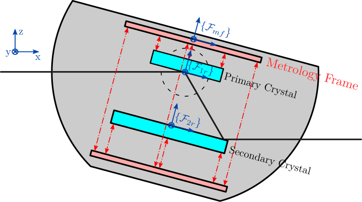
Figure 1: Schematic of the DCM with one set of first and second crystals with the associated frames
Here are the different letters used in the notations and there meaning:
r: “ring” (i.e. toward \(-y\))h: “hall” (i.e. toward \(+y\))u: “upstream” (i.e. towards \(-x\))d: “downstream” (i.e. towards \(+x\))c: “center” (i.e. centered at \(x=0\))1: primary crystal2: secondary crystalmf: metrology frame
2. Forward and Inverse Kinematics problems
Let’s consider one plane initially orthogonal to the \(z\) direction (Figure 2). The pose of the plane, expressed in a frame \(\{\mathcal{F}\}\) with origin \(\mathcal{O}\) is defined by:
- its vertical motion: \(d_z\)
- its rotation around the \(y\) axis: \(r_y\)
- its rotation around the \(x\) axis: \(r_x\)
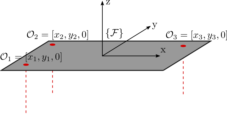
Figure 2: SChematic of a plane with three vertical interferometers
In order to measure the pose of the crystal, three interferometers are measuring the motion of the plane at three distinct positions \(\mathcal{O}_1 = [x_1, y_1, 0]\), \(\mathcal{O}_2 = [x_2, y_2, 0]\) and \(\mathcal{O}_3 = [x_3, y_3, 0]\) (See Figure 2). The interferometers can be pointed in the \(z\) direction or in the opposite \(z\) direction. The measured motion are noted \(z_1\), \(z_2\) and \(z_3\).
The inverse kinematic problem consists of deriving the measured \([z_1, z_2, z_3]\) motions from the pose \([d_z, r_y, r_x]\) of the crystal. For small motion, this problem can be easily solved as follows:
\begin{equation} \boxed{ \begin{bmatrix} z_{1} \\ z_{2} \\ z_{3} \end{bmatrix} = \bm{J} \begin{bmatrix} d_{z} \\ r_{y} \\ r_{x} \end{bmatrix} } \end{equation}with \(\bm{J}\) called the Jacobian matrix.
The Jacobian matrix can be computed as follows in the case where the interferometers are pointing toward positive \(z\):
\begin{equation} \label{eq:jacobian_3dof_positive_z} \boxed{ \bm{J} = \begin{bmatrix} 1 & -x_1 & y_1 \\ 1 & -x_2 & y_2 \\ 1 & -x_3 & y_3 \end{bmatrix} } \end{equation}and computed as follows if there are pointing torward negative \(z\):
\begin{equation} \label{eq:jacobian_3dof_negative_z} \boxed{ \bm{J} = \begin{bmatrix} -1 & x_1 & -y_1 \\ -1 & x_2 & -y_2 \\ -1 & x_3 & -y_3 \end{bmatrix} } \end{equation}The forward kinematic problem is then solved by inverting the Jacobian matrix:
\begin{equation} \boxed{ \begin{bmatrix} d_{z} \\ r_{y} \\ r_{x} \end{bmatrix} = \bm{J}^{-1} \begin{bmatrix} z_{1} \\ z_{2} \\ z_{3} \end{bmatrix} } \end{equation}The same reasoning can be performed to convert the wanted motion of one plane to the motion of three vertical actuators fixed to the plane (tripod architecture).
3. Bragg Angle
In order to have a fix exit, the following relation must be verified:
\begin{equation} \label{eq:bragg_angle_formula} \boxed{d_z = \frac{d_{\text{off}}}{2 \cos \theta_b}} \end{equation}with:
- \(d_{\text{off}}\) the wanted offset between the incident x-ray and the output x-ray
- \(\theta_b\) the bragg angle
- \(d_z\) the corresponding distance between the first and second crystal
This relation is shown in Figure 3 for a wanted fix exit offset of 10mm.
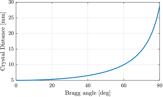
Figure 3: Jack motion as a function of Bragg angle (\(d_z = 10\,mm\))
4. Kinematics of “hall” Crystals
4.1. Interferometers - Primary “Hall” Crystal
Three interferometers fixed to the top metrology frame are pointed to the top surface (i.e. toward negative \(z\)) of the primary “hall” crystal. The measurements are performed along the \(z\) direction.
The notations are:
- \(\{\mathcal{F}_{1h}\}\) is the frame in which motion of the crystal are expressed
- \(\mathcal{O}_{1h,u}\) measurement point for the “upstream” interferometer
- \(\mathcal{O}_{1h,c}\) measurement point for the “center” interferometer
- \(\mathcal{O}_{1h,d}\) measurement point for the “downstream” interferometer
The measured displacements by the interferometers are noted \([z_{1h,u},\ z_{1h,c},\ z_{1h,d}]\).
The corresponding motion of the crystal expressed in the frame as shown in Figure 4 are:
- \(d_{1h,z}\) motion in the \(z\) direction
- \(r_{1h,y}\) rotation around the \(y\) axis
- \(r_{1h,x}\) rotation around the \(x\) axis

Figure 4: Top view of the primary crystal hall. Position of the measurement points. Units in [mm]
The inverse kinematics problem consists of deriving the measured displacement by the interferometer from the motion of the crystal (see Figure 5):
\begin{equation} \boxed{ \begin{bmatrix} z_{1h,u} \\ z_{1h,c} \\ z_{1h,d} \end{bmatrix} = \bm{J}_{1h,s} \begin{bmatrix} d_{1h,z} \\ r_{1h,y} \\ r_{1h,x} \end{bmatrix} } \end{equation}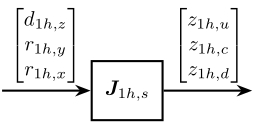
Figure 5: Inverse Kinematics - Interferometers
From the measurement coordinates in Figure 4 and equation eq:jacobian_3dof_negative_z, the inverse kinematics the folowing Jacobian matrix is obtained:
\begin{equation} \boxed{\bm{J}_{1h,s} = \begin{bmatrix} -1 & -0.036 & 0.015 \\ -1 & 0 & -0.015 \\ -1 & 0.036 & 0.015 \end{bmatrix}} \end{equation}The forward kinematics problem (computing the crystal motion from the 3 interferometers) is solved by inverting the Jacobian matrix (see Figure 6).
\begin{equation} \boxed{ \begin{bmatrix} d_{1h,z} \\ r_{1h,y} \\ r_{1h,x} \end{bmatrix} = \bm{J}_{1h,s}^{-1} \begin{bmatrix} z_{1h,ur} \\ z_{1h,ch} \\ z_{1h,dr} \end{bmatrix} } \end{equation}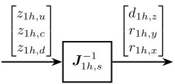
Figure 6: Forward Kinematics - Interferometers
The obtained matrix is displayed in Table 1.
| -0.25 | -0.5 | -0.25 |
| -13.89 | 0.0 | 13.89 |
| 16.67 | -33.33 | 16.67 |
4.2. Interferometers - Secondary “Hall” Crystal
Three interferometers are pointed to the bottom surface (i.e. toward positive \(z\)) of the secondary “hall” crystal.
The position of the measurement points are shown in Figure 7 as well as the origin where the motion of the crystal is computed.
The notations are:
- \(\{\mathcal{F}_{2h}\}\) is the frame in which motion of the crystal are expressed
- \(\mathcal{O}_{2h,u}\) measurement point for the “upstream” interferometer
- \(\mathcal{O}_{2h,c}\) measurement point for the “center” interferometer
- \(\mathcal{O}_{2h,d}\) measurement point for the “downstream” interferometer
The measured displacements by the interferometers are noted \([z_{2h,u},\ z_{2h,c},\ z_{2h,d}]\).
The corresponding motion of the crystal expressed in the frame as shown in Figure 7 are:
- \(d_{2h,z}\) motion in the \(z\) direction
- \(r_{2h,y}\) rotation around the \(y\) axis
- \(r_{2h,x}\) rotation around the \(x\) axis

Figure 7: Bottom view of the secondary “hall” crystal. Position of the measurement points. Coordinate values are in [mm]
The inverse kinematics consisting of deriving the interferometer measurements from the motion of the crystal (see Figure 8):
\begin{equation} \boxed{ \begin{bmatrix} z_{2h,u} \\ z_{2h,c} \\ z_{2h,d} \end{bmatrix} = \bm{J}_{2h,s} \begin{bmatrix} d_{2h,z} \\ r_{2h,y} \\ r_{2h,x} \end{bmatrix} } \end{equation}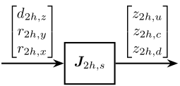
Figure 8: Inverse Kinematics - Interferometers
From the measurement coordinates in Figure 7 and equation eq:jacobian_3dof_positive_z, the inverse kinematics the folowing Jacobian matrix is obtained:
\begin{equation} \boxed{\bm{J}_{2h,s} = \begin{bmatrix} 1 & 0.07 & -0.015 \\ 1 & 0 & 0.015 \\ 1 & -0.07 & -0.015 \end{bmatrix}} \end{equation}The forward kinematics is solved by inverting the Jacobian matrix (see Figure 9).
\begin{equation} \boxed{ \begin{bmatrix} d_{2h,z} \\ r_{2h,y} \\ r_{2h,x} \end{bmatrix} = \bm{J}_{2h,s}^{-1} \begin{bmatrix} z_{2h,u} \\ z_{2h,c} \\ z_{2h,d} \end{bmatrix} } \end{equation}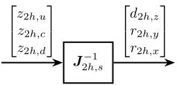
Figure 9: Forward Kinematics - Interferometers
The results is shown in Table 2.
| 0.25 | 0.5 | 0.25 |
| 7.14 | 0.0 | -7.14 |
| -16.67 | 33.33 | -16.67 |
4.3. Piezo - hall Crystal
The locations of the actuators with respect with the center of the secondary “hall” crystal are shown in Figure 10.
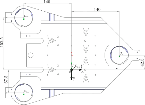
Figure 10: Location of actuators with respect to the center of the hall second crystal (bottom view). Units are in [mm]
Inverse Kinematics consist of deriving the corresponding z motion of the 3 actuators from the motion of the crystal expressed in \(\{\mathcal{F}_{2h}\}\). As in the previous section, the motion of the secondary “hall” crystal is expressed by \([d_{2h,z},\ r_{2h,y},\ r_{2h,x}]\). The motion of the three fast jacks are expressed by \([d_{u_r},\ d_{u_h},\ d_{d}]\) are are corresponding to a motion along the \(z\) axis toward positive values.
The inverse kinematics can therefore be solved as follows:
\begin{equation} \boxed{ \begin{bmatrix} d_{u_r} \\ d_{u_h} \\ d_{d} \end{bmatrix} = \bm{J}_{h,a} \begin{bmatrix} d_{2h,z} \\ r_{2h,y} \\ r_{2h,x} \end{bmatrix} } \end{equation}
Figure 11: Inverse Kinematics - Actuators
Based on the geometry in Figure 10, the following Jacobian matrix is obtained (see Eq. eq:jacobian_3dof_positive_z):
\begin{equation} \boxed{\bm{J}_{h,a} = \begin{bmatrix} 1 & 0.14 & -0.1525 \\ 1 & 0.14 & 0.0675 \\ 1 & -0.14 & -0.0425 \end{bmatrix}} \end{equation}The forward Kinematics is solved by inverting the Jacobian matrix:
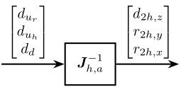
\begin{equation} \boxed{ \begin{bmatrix} d_{2h,z} \\ r_{2h,y} \\ r_{2h,x} \end{bmatrix} = \bm{J}_{h,a}^{-1} \begin{bmatrix} d_{u_r} \\ d_{u_h} \\ d_{d} \end{bmatrix} } \end{equation}
 The obtained inverse Jacobian matrix is shown in Table 3.
| 0.0568 | 0.4432 | 0.5 |
| 1.7857 | 1.7857 | -3.5714 |
| -4.5455 | 4.5455 | 0.0 |
5. Kinematics of “ring” Crystals
5.1. Interferometers - ring primary Crystal
Three interferometers fixed to the top metrology frame are pointed to the top surface (i.e. toward negative \(z\)) of the primary “hall” crystal. The measurements are perform along the \(z\) direction.
The notations are:
- \(\{\mathcal{F}_{1r}\}\) is the frame in which motion of the crystal are expressed
- \(\mathcal{O}_{1r,u}\) measurement point for the “upstream” interferometer
- \(\mathcal{O}_{1r,c}\) measurement point for the “center” interferometer
- \(\mathcal{O}_{1r,d}\) measurement point for the “downstream” interferometer
The measured displacements by the interferometers are noted \([z_{1r,u},\ z_{1r,c},\ z_{1r,d}]\).
The corresponding motion of the crystal expressed in the frame as shown in Figure 4 are:
- \(d_{1r,z}\) motion in the \(z\) direction
- \(r_{1r,y}\) rotation around the \(y\) axis
- \(r_{1r,x}\) rotation around the \(x\) axis

Figure 12: Top view of the primary crystal ring. Position of the measurement points in [mm].
The inverse kinematics consisting of deriving the interferometer measurements from the motion of the crystal (see Figure 13):
\begin{equation} \boxed{ \begin{bmatrix} z_{1r,u} \\ z_{1r,c} \\ z_{1r,d} \end{bmatrix} = \bm{J}_{1r,s} \begin{bmatrix} d_{1r,z} \\ r_{1r,y} \\ r_{1r,x} \end{bmatrix} } \end{equation}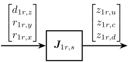
Figure 13: Inverse Kinematics - Interferometers (primary “ring” crystal)
From the measurement coordinates in Figure 12 and equation eq:jacobian_3dof_negative_z, the inverse kinematics the folowing Jacobian matrix is obtained:
\begin{equation} \boxed{\bm{J}_{1r,s} = \begin{bmatrix} -1 & -0.036 & -0.015 \\ -1 & 0 & 0.015 \\ -1 & 0.036 & -0.015 \end{bmatrix}} \end{equation}The forward kinematics is solved by inverting the Jacobian matrix (see Figure 14).
\begin{equation} \boxed{ \begin{bmatrix} d_{1r,z} \\ r_{1r,y} \\ r_{1r,x} \end{bmatrix} = \bm{J}_{1r,s}^{-1} \begin{bmatrix} z_{1r,u} \\ z_{1r,c} \\ z_{1r,d} \end{bmatrix} } \end{equation}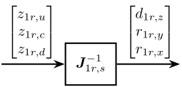
Figure 14: Forward Kinematics - Interferometers
The obtained inverse Jacobian matrix is shown in Table 4.
| -0.25 | -0.5 | -0.25 |
| -13.89 | 0.0 | 13.89 |
| -16.67 | 33.33 | -16.67 |
5.2. Interferometers - ring secondary Crystal
Three interferometers are pointed to the bottom surface (i.e. toward positive \(z\)) of the secondary “ring” crystal.
The position of the measurement points are shown in Figure 15 as well as the origin where the motion of the crystal is computed.
The notations are:
- \(\{\mathcal{F}_{2r}\}\) is the frame in which motion of the crystal are expressed
- \(\mathcal{O}_{2r,u}\) measurement point for the “upstream” interferometer
- \(\mathcal{O}_{2r,c}\) measurement point for the “center” interferometer
- \(\mathcal{O}_{2r,d}\) measurement point for the “downstream” interferometer
The measured displacements by the interferometers are noted \([z_{2r,u},\ z_{2r,c},\ z_{2r,d}]\).
The corresponding motion of the crystal expressed in the frame as shown in Figure 7 are:
- \(d_{2r,z}\) motion in the \(z\) direction
- \(r_{2r,y}\) rotation around the \(y\) axis
- \(r_{2r,x}\) rotation around the \(x\) axis
The position of the measurement points are shown in Figure 15 as well as the origin where the motion of the crystal is computed.

Figure 15: Bottom view of the second crystal ring. Position of the measurement points.
The inverse kinematics consisting of deriving the interferometer measurements from the motion of the crystal (see Figure 16):
\begin{equation} \boxed{ \begin{bmatrix} z_{2r,u} \\ z_{2r,c} \\ z_{2r,d} \end{bmatrix} = \bm{J}_{2r,s} \begin{bmatrix} d_{2r,z} \\ r_{2r,y} \\ r_{2r,x} \end{bmatrix} } \end{equation}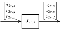
Figure 16: Inverse Kinematics - Interferometers
From the measurement coordinates in Figure 15 and equation eq:jacobian_3dof_positive_z, the inverse kinematics the folowing Jacobian matrix is obtained:
\begin{equation} \boxed{\bm{J}_{2r,s} = \begin{bmatrix} 1 & 0.07 & 0.015 \\ 1 & 0 & -0.015 \\ 1 & -0.07 & 0.015 \end{bmatrix}} \end{equation}The forward kinematics is solved by inverting the Jacobian matrix (see Figure 17).
\begin{equation} \boxed{ \begin{bmatrix} d_{2r,z} \\ r_{2r,y} \\ r_{2r,x} \end{bmatrix} = \bm{J}_{2r,s}^{-1} \begin{bmatrix} z_{2r,u} \\ z_{2r,c} \\ z_{2r,d} \end{bmatrix} } \end{equation}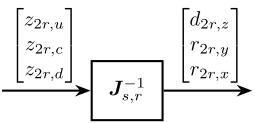
Figure 17: Forward Kinematics - Interferometers
The obtained inverse Jacobian matrix is shown in Table 5.
| 0.25 | 0.5 | 0.25 |
| 7.14 | 0.0 | -7.14 |
| 16.67 | -33.33 | 16.67 |
5.3. Piezo - ring Crystal
The location of the actuators with respect with the center of the secondary “ring” crystal are shown in Figure 18.
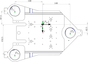
Figure 18: Location of actuators with respect to the center of the ring second crystal (bottom view)
Inverse Kinematics consist of deriving the corresponding z motion of the 3 actuators from the motion of the crystal expressed in \(\{\mathcal{F}_{2r}\}\). As in the previous section, the motion of the secondary “ring” crystal is expressed by \([d_{2r,z},\ r_{2r,y},\ r_{2r,x}]\). The motion of the three fast jacks are expressed by \([d_{u_r},\ d_{u_h},\ d_{d}]\) are are corresponding to a motion along the \(z\) axis toward positive values.
The inverse kinematics can therefore be solved as follows:
\begin{equation} \boxed{ \begin{bmatrix} d_{u_r} \\ d_{u_h} \\ d_{d} \end{bmatrix} = \bm{J}_{h,a} \begin{bmatrix} d_{2r,z} \\ r_{2r,y} \\ r_{2r,x} \end{bmatrix} } \end{equation}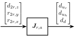
Figure 19: Inverse Kinematics - Actuators
Based on the geometry in Figure 18, we obtain (see Eq. eq:jacobian_3dof_positive_z):
\begin{equation} \boxed{\bm{J}_{r,a} = \begin{bmatrix} 1 & 0.14 & -0.0675 \\ 1 & 0.14 & 0.1525 \\ 1 & -0.14 & 0.0425 \end{bmatrix}} \end{equation}The forward Kinematics is solved by inverting the Jacobian matrix:
\begin{equation} \boxed{ \begin{bmatrix} d_{2r,z} \\ r_{2r,y} \\ r_{2r,x} \end{bmatrix} = \bm{J}_{r,a}^{-1} \begin{bmatrix} d_{u_r} \\ d_{u_h} \\ d_{d} \end{bmatrix} } \end{equation}
Figure 20: Forward Kinematics - Actuators for ring crystal
The obtained inverse Jacobian matrix is shown in Table 6.
| 0.4432 | 0.0568 | 0.5 |
| 1.7857 | 1.7857 | -3.5714 |
| -4.5455 | 4.5455 | 0.0 |
6. Kinematics of the Metrology Frame
Three interferometers (aligned with the \(z\) axis) are used to measure the relative motion between the bottom part and the top part of the metrology frame.
The location of the three interferometers are shown in Figure 21.
The measured displacements by the interferometers are are noted \([z_{mf,u},\ z_{mf,dh},\ z_{mf,dr}]\).
We here suppose that the bottom part of the metrology frame is fixed and only the top part is moving. The motion of the metrology top part expressed in the frame as shown in Figure 21 are:
- \(d_{mf,z}\) motion in the \(z\) direction
- \(r_{mf,y}\) rotation around the \(y\) axis
- \(r_{mf,x}\) rotation around the \(x\) axis
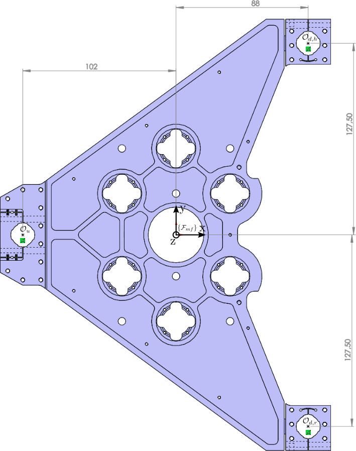
Figure 21: Top View of the top part of the metrology frame
The inverse kinematics consisting of deriving the interferometer measurements from the motion of the metrology top part:
\begin{equation} \boxed{ \begin{bmatrix} z_{mf,u} \\ z_{mf,dh} \\ z_{mf,dr} \end{bmatrix} = \bm{J}_{mf,s} \begin{bmatrix} d_{mf,z} \\ r_{mf,y} \\ r_{mf,x} \end{bmatrix} } \end{equation}From the coordinates in Figure 21 and the equation eq:jacobian_3dof_positive_z, the following Jacobian matrix is obtained:
\begin{equation} \boxed{\bm{J}_{mf,r} = \begin{bmatrix} 1 & 0.102 & 0 \\ 1 & -0.088 & 0.1275 \\ 1 & -0.088 & -0.1275 \end{bmatrix}} \end{equation}The forward kinematics is solved by inverting the Jacobian matrix:
\begin{equation} \boxed{ \begin{bmatrix} d_{mf,z} \\ r_{mf,y} \\ r_{mf,x} \end{bmatrix} = \bm{J}_{mf,s}^{-1} \begin{bmatrix} z_{mf,u} \\ z_{mf,dh} \\ z_{mf,dr} \end{bmatrix} } \end{equation}The obtained inverse Jacobian matrix is shown in Table 7.
| 0.463 | 0.268 | 0.268 |
| 5.263 | -2.632 | -2.632 |
| 0.0 | 3.922 | -3.922 |
7. Computing relative position between Crystals
In the previous sections, the motion of the individual crystals have been computed.
We wish to express the relative pose of the primary and secondary crystals \([d_{h,z},\ r_{h,y},\ r_{h,x}]\) or \([d_{r,z},\ r_{r,y},\ r_{r,x}]\).
The sign conventions for the relative crystal pose are:
- An increase of \(d_{h,z}\) means the two crystals are further apart
- An increase of \(r_{h,}\) means that the second crystals experiences a rotation around \(y\) with respect to the primary crystal
- An increase of \(r_{h,x}\) means that the second crystals experiences a rotation around \(x\) with respect to the primary crystal
We therefore have the following relation (same for “hall” and “ring” crystals):
\begin{equation} \boxed{ \begin{bmatrix} d_{h,z} \\ r_{h,y} \\ r_{h,x} \end{bmatrix} = \begin{bmatrix} d_{2h,z} \\ r_{2h,y} \\ r_{2h,x} \end{bmatrix} - \begin{bmatrix} d_{1h,z} \\ r_{1h,y} \\ r_{1h,x} \end{bmatrix} - \begin{bmatrix} d_{mf,z} \\ r_{mf,y} \\ r_{mf,x} \end{bmatrix} } \end{equation}The relative pose can be expressed as a function of the interferometers using the Jacobian matrices for the “hall” crystals:
\begin{equation} \boxed{ \begin{bmatrix} d_{h,z} \\ r_{h,y} \\ r_{h,x} \end{bmatrix} = \bm{J}_{2h,s}^{-1} \begin{bmatrix} z_{2h,u} \\ z_{2h,c} \\ z_{2h,d} \end{bmatrix} - \bm{J}_{1h,s}^{-1} \begin{bmatrix} z_{1h,u} \\ z_{1h,c} \\ z_{1h,d} \end{bmatrix} - \bm{J}_{mf,s}^{-1} \begin{bmatrix} z_{mf,u} \\ z_{mf,dh} \\ z_{mf,dr} \end{bmatrix} } \end{equation}As well as for the “ring” crystals:
\begin{equation} \boxed{ \begin{bmatrix} d_{r,z} \\ r_{r,y} \\ r_{r,x} \end{bmatrix} = \bm{J}_{2r,s}^{-1} \begin{bmatrix} z_{2r,u} \\ z_{2r,c} \\ z_{2r,d} \end{bmatrix} - \bm{J}_{1r,s}^{-1} \begin{bmatrix} z_{1r,u} \\ z_{1r,c} \\ z_{1r,d} \end{bmatrix} - \bm{J}_{mf,s}^{-1} \begin{bmatrix} z_{mf,u} \\ z_{mf,dr} \\ z_{mf,dr} \end{bmatrix} } \end{equation}8. Summary - List of notations
There are 5 Jacobian matrices that are used to convert the 15 interferometers to the relative pose between the primary and secondary crystals as well as 2 Jacobian matrices for the actuators. All Jacobian matrices are summarized in Table 8.
| Notation | Variable | Description |
|---|---|---|
| \(\bm{J}_{1h,s}\) | J_1h_s |
Converts interferometers to the first “hall” crystal pose |
| \(\bm{J}_{2h,s}\) | J_2h_s |
Converts interferometers to the second “hall” crystal pose |
| \(\bm{J}_{1r,s}\) | J_1r_s |
Converts interferometers to the first “ring” crystal pose |
| \(\bm{J}_{2r,s}\) | J_2r_s |
Converts interferometers to the second “ring” crystal pose |
| \(\bm{J}_{mf,s}\) | J_mf_s |
Converts interferometers to the first “hall” crystal pose |
| \(\bm{J}_{h,a}\) | J_h_a |
Converts Fastjack motion to the second “hall” crystal pose |
| \(\bm{J}_{r,a}\) | J_r_a |
Converts Fastjack motion to the second “ring” crystal pose |
The 15 interferometer measurements are summarized in Table 9.
| Notation | Variable | Interferometer |
|---|---|---|
| \(z_{1h,u}\) | z_1h_u |
First “Hall” Crystal, “upstream” |
| \(z_{1h,c}\) | z_1h_c |
First “Hall” Crystal, “center” |
| \(z_{1h,d}\) | z_1h_d |
First “Hall” Crystal, “downstream” |
| \(z_{2h,u}\) | z_2h_u |
Second “Hall” Crystal, “upstream” |
| \(z_{2h,c}\) | z_2h_c |
Second “Hall” Crystal, “center” |
| \(z_{2h,d}\) | z_2h_d |
Second “Hall” Crystal, “downstream” |
| \(z_{1r,u}\) | z_1r_u |
First “Ring” Crystal, “upstream” |
| \(z_{1r,c}\) | z_1r_c |
First “Ring” Crystal, “center” |
| \(z_{1r,d}\) | z_1r_d |
First “Ring” Crystal, “downstream” |
| \(z_{2r,u}\) | z_2r_u |
Second “Ring” Crystal, “upstream” |
| \(z_{2r,c}\) | z_2r_c |
Second “Ring” Crystal, “center” |
| \(z_{2r,d}\) | z_2r_d |
Second “Ring” Crystal, “downstream” |
| \(z_{mf,u}\) | z_mf_u |
Metrology Frame, “upstream” |
| \(z_{mf,dh}\) | z_mf_dh |
Metrology Frame, “downstream-hall” |
| \(z_{mf,dr}\) | z_mf_dr |
Metrology Frame, “downstream-ring” |
From the 15 interferometers, several crystal pose are computed. They are summarized in Table 10.
| Notation | Variable | Description |
|---|---|---|
| \(d_{1h,z}\) | d_1h_z |
First “Hall” Crystal, z-translation |
| \(r_{1h,y}\) | r_1h_y |
First “Hall” Crystal, y-rotation |
| \(r_{1h,x}\) | r_1h_x |
First “Hall” Crystal, x-rotation |
| \(d_{2h,z}\) | d_2h_z |
Second “Hall” Crystal, z-translation |
| \(r_{2h,y}\) | r_2h_y |
Second “Hall” Crystal, y-rotation |
| \(r_{2h,x}\) | r_2h_x |
Second “Hall” Crystal, x-rotation |
| \(d_{1r,z}\) | d_1r_z |
First “Ring” Crystal, z-translation |
| \(r_{1r,y}\) | r_1r_y |
First “Ring” Crystal, y-rotation |
| \(r_{1r,x}\) | r_1r_x |
First “Ring” Crystal, x-rotation |
| \(d_{2r,z}\) | d_2r_z |
Second “Ring” Crystal, z-translation |
| \(r_{2r,y}\) | r_2r_y |
Second “Ring” Crystal, y-rotation |
| \(r_{2r,x}\) | r_2r_x |
Second “Ring” Crystal, x-rotation |
| \(d_{mf,z}\) | d_mf_z |
Metrology Frame, z-translation (top relative to bottom) |
| \(r_{mf,y}\) | r_mf_y |
Metrology Frame, y-rotation (top relative to bottom) |
| \(r_{mf,x}\) | r_mf_x |
Metrology Frame, x-rotation (top relative to bottom) |
And finally, the relative pose between the first and second crystals are defined in Table 11.
| Notation | Variable | Description |
|---|---|---|
| \(d_{h,z}\) | d_h_z |
Relative distance between the “hall” crystals |
| \(r_{h,y}\) | r_h_y |
Relative y-rotation of the 2nd “hall” crystal w.r.t. the primary |
| \(r_{h,x}\) | r_h_x |
Relative x-rotation of the 2nd “hall” crystal w.r.t. the primary |
| \(d_{r,z}\) | d_r_z |
Relative distance between the “ring” crystals |
| \(r_{r,y}\) | r_r_y |
Relative y-rotation of the 2nd “ring” crystal w.r.t. the primary |
| \(r_{r,x}\) | r_r_x |
Relative x-rotation of the 2nd “ring” crystal w.r.t. the primary |
9. Save Kinematics
All the Jacobian matrix are exported so that there can be easily imported for computation purposes.
save('mat/dcm_kinematics.mat', 'J_1h_s', 'J_1r_s', 'J_2h_s', 'J_2r_s', 'J_mf_s', 'J_h_a', 'J_r_a')