ESRF Double Crystal Monochromator - Feedback Controller
Table of Contents
This report is also available as a pdf.
1. Estimation of Sensitivity Function
1.1. Load Data
Two scans are performed:
1.1in mode B3.1in mode C
The difference between the two is that mode C adds the feedback controller.
%% Load Data of the new LUT method
Ts = 0.1;

ol_drx = 1e-9*double(h5read('xanes_0003.h5','/1.1/measurement/xtal_111_drx_filter')); % Rx [rad]
cl_drx = 1e-9*double(h5read('xanes_0003.h5','/3.1/measurement/xtal_111_drx_filter')); % Rx [rad]

ol_dry = 1e-9*double(h5read('xanes_0003.h5','/1.1/measurement/xtal_111_dry_filter')); % Ry [rad]
cl_dry = 1e-9*double(h5read('xanes_0003.h5','/3.1/measurement/xtal_111_dry_filter')); % Ry [rad]

t = linspace(Ts, Ts*length(ol_drx), length(ol_drx));
By comparison the frequency content of the crystal orientation errors between mode B and mode C, it is possible to estimate the Sensitivity transfer function (Figure 1).
win = hanning(ceil(1/Ts));

[pxx_ol_drx, f] = pwelch(ol_drx, win, [], [], 1/Ts);
[pxx_cl_drx, ~] = pwelch(cl_drx, win, [], [], 1/Ts);

[pxx_ol_dry, ~] = pwelch(ol_dry, win, [], [], 1/Ts);
[pxx_cl_dry, ~] = pwelch(cl_dry, win, [], [], 1/Ts);
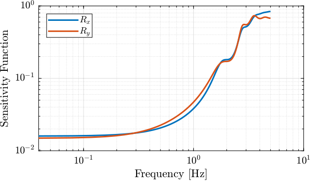
Figure 1: Estimation of the sensitivity transfer function magnitude
1.2. Controller
load('X_tal_cage_PID.mat', 'K');
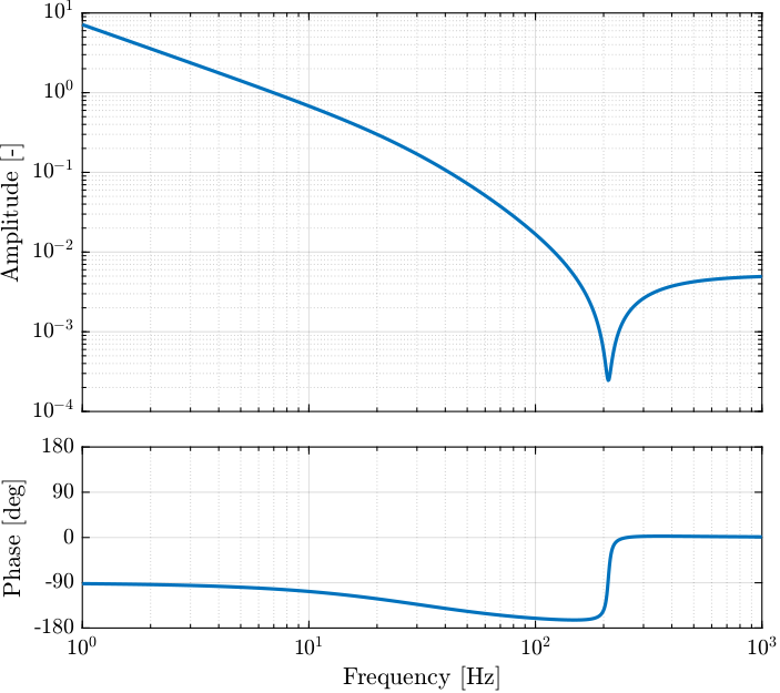
Figure 2: Bode Plot of the Controller
1.3. Test
Ts = 5e-3;
cl_drx = 1e-9*double(h5read('xanes_0003.h5','/16.1/measurement/xtal_111_drx_filter')); % Rx [rad]
ol_drx = 1e-9*double(h5read('xanes_0003.h5','/18.1/measurement/xtal_111_drx_filter')); % Rx [rad]

t = linspace(Ts, Ts*length(ol_drx), length(ol_drx));
figure;
hold on;
plot(t, ol_drx)
plot(t, cl_drx)
win = hanning(ceil(10/Ts));

[pxx_ol_drx, f] = pwelch(ol_drx, win, [], [], 1/Ts);
[pxx_cl_drx, ~] = pwelch(cl_drx, win, [], [], 1/Ts);
2. System Identification
2.1. Identification ID24
load('test_id_id24_3.mat')
t = 1e-4*ones(size(fjpur, 1), 1);

ur.dz  = fjpur(:,1) - mean(fjpur(:,1));
ur.dry = fjpur(:,2) - mean(fjpur(:,2));
ur.drx = fjpur(:,3) - mean(fjpur(:,3));
ur.u   = fjpur(:,7) - mean(fjpur(:,7));

uh.dz  = fjpuh(:,1) - mean(fjpuh(:,1));
uh.dry = fjpuh(:,2) - mean(fjpuh(:,2));
uh.drx = fjpuh(:,3) - mean(fjpuh(:,3));
uh.u   = fjpuh(:,8) - mean(fjpuh(:,8));

d.dz  = fjpd(:,1) - mean(fjpd(:,1));
d.dry = fjpd(:,2) - mean(fjpd(:,2));
d.drx = fjpd(:,3) - mean(fjpd(:,3));
d.u   = fjpd(:,9) - mean(fjpd(:,9));
J_a_311 = [1,  0.14, -0.0675
           1,  0.14,  0.1525
           1, -0.14,  0.0425];

J_a_111 = [1,  0.14, -0.1525
           1,  0.14,  0.0675
           1, -0.14, -0.0425];

ur.y = [J_a_311 * [-ur.dz, ur.dry,-ur.drx]']';
uh.y = [J_a_311 * [-uh.dz, uh.dry,-uh.drx]']';
d.y  = [J_a_311 * [-d.dz,  d.dry, -d.drx]']';
%% Sampling Time and Frequency
Ts = 1e-4; % [s]
Fs = 1/Ts; % [Hz]

% Hannning Windows
win = hanning(ceil(1*Fs));
%% And we get the frequency vector
[G_ur, f] = tfestimate(ur.u, ur.y, win, [], [], 1/Ts);
[G_uh, ~] = tfestimate(uh.u, uh.y, win, [], [], 1/Ts);
[G_d,  ~] = tfestimate(d.u,  d.y,  win, [], [], 1/Ts);
[coh_ur, ~] = mscohere(ur.u, ur.y, win, [], [], 1/Ts);
[coh_uh, ~] = mscohere(uh.u, uh.y, win, [], [], 1/Ts);
[coh_d,  ~] = mscohere(d.u,  d.y,  win, [], [], 1/Ts);
2.2. Identification
ur = load('FJPUR_step.mat');
uh = load('FJPUH_step.mat');
d  = load('FJPD_step.mat');
| 1 | dz311 |
| 2 | dry311 |
| 3 | drx311 |
| 4 | dz111 |
| 5 | dry111 |
| 6 | drx111 |
| 7 | fjpur |
| 8 | fjpuh |
| 9 | fjpd |
| 10 | bragg |
ur.time = ur.time - ur.time(1);
ur.allValues(:, 1) = ur.allValues(:, 1) - mean(ur.allValues(ur.time<1, 1));
ur.allValues(:, 2) = ur.allValues(:, 2) - mean(ur.allValues(ur.time<1, 2));
ur.allValues(:, 3) = ur.allValues(:, 3) - mean(ur.allValues(ur.time<1, 3));

t_filt = ur.time > 48 & ur.time < 60;

ur.u = ur.allValues(t_filt, 7);
ur.y_111 = [-ur.allValues(t_filt, 1), ur.allValues(t_filt, 2), ur.allValues(t_filt, 3)];
uh.time = uh.time - uh.time(1);
uh.allValues(:, 1) = uh.allValues(:, 1) - mean(uh.allValues(uh.time<1, 1));
uh.allValues(:, 2) = uh.allValues(:, 2) - mean(uh.allValues(uh.time<1, 2));
uh.allValues(:, 3) = uh.allValues(:, 3) - mean(uh.allValues(uh.time<1, 3));

uh.u = uh.allValues(t_filt, 8);
uh.y_111 = [-uh.allValues(t_filt, 1), uh.allValues(t_filt, 2), uh.allValues(t_filt, 3)];
d.time = d.time - d.time(1);
d.allValues(:, 1) = d.allValues(:, 1) - mean(d.allValues(d.time<1, 1));
d.allValues(:, 2) = d.allValues(:, 2) - mean(d.allValues(d.time<1, 2));
d.allValues(:, 3) = d.allValues(:, 3) - mean(d.allValues(d.time<1, 3));

d.u = d.allValues(t_filt, 9);
d.y_111 = [-d.allValues(t_filt, 1), d.allValues(t_filt, 2), d.allValues(t_filt, 3)];
J_a_111 = [1,  0.14, -0.0675
           1,  0.14,  0.1525
           1, -0.14,  0.0425];

J_a_311 = [1,  0.14, -0.1525
           1,  0.14,  0.0675
           1, -0.14, -0.0425];

ur.y = [J_a_311 * ur.y_111']';
uh.y = [J_a_311 * uh.y_111']';
d.y  = [J_a_311 * d.y_111']';
%% Sampling Time and Frequency
Ts = 1e-4; % [s]
Fs = 1/Ts; % [Hz]

% Hannning Windows
win = hanning(ceil(5*Fs));
%% And we get the frequency vector
[G_ur, f] = tfestimate(ur.u, ur.y, win, [], [], 1/Ts);
[G_uh, ~] = tfestimate(uh.u, uh.y, win, [], [], 1/Ts);
[G_d,  ~] = tfestimate(d.u,  d.y,  win, [], [], 1/Ts);
[coh_ur, ~] = mscohere(ur.u, ur.y, win, [], [], 1/Ts);
[coh_uh, ~] = mscohere(uh.u, uh.y, win, [], [], 1/Ts);
[coh_d,  ~] = mscohere(d.u,  d.y,  win, [], [], 1/Ts);
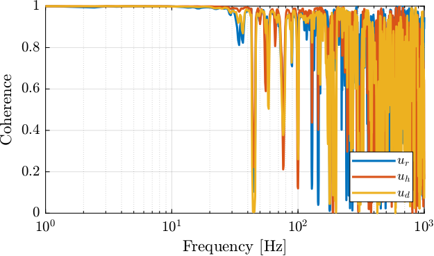
Figure 3: Coherence
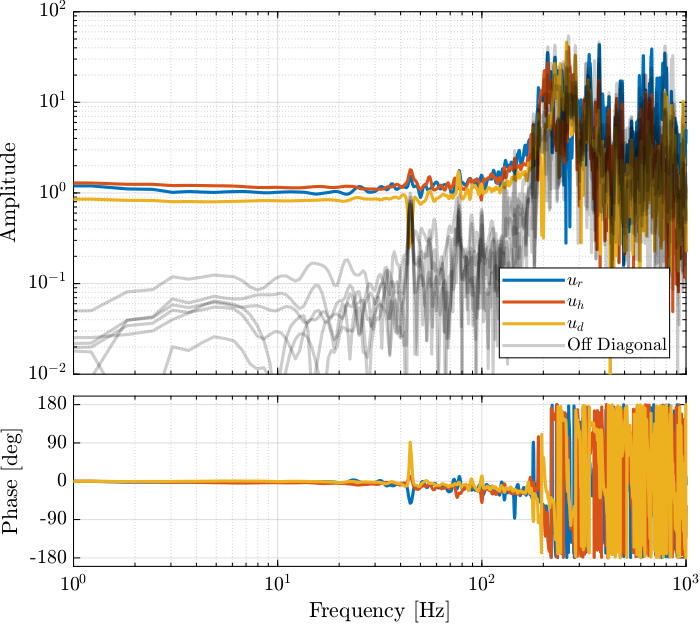
Figure 4: Bode Plot of the DCM dynamics in the frame of the fast jack.
%% Previously used controller
load('X_tal_cage_PID.mat', 'K');
%% Controller design
s = tf('s');

% Lead
a  = 4;  % Amount of phase lead / width of the phase lead / high frequency gain
wc = 2*pi*20; % Frequency with the maximum phase lead [rad/s]

% Low Pass Filter
w0 = 2*pi*100; % Cut-off frequency [rad/s]
xi = 0.4; % Damping Ratio

Kb = eye(3)*(2*pi*20)^2/(s^2) *1/(sqrt(a))* (1 + s/(wc/sqrt(a)))/(1 + s/(wc*sqrt(a))) * 1/(1 + 2*xi/w0*s + s^2/w0^2);;
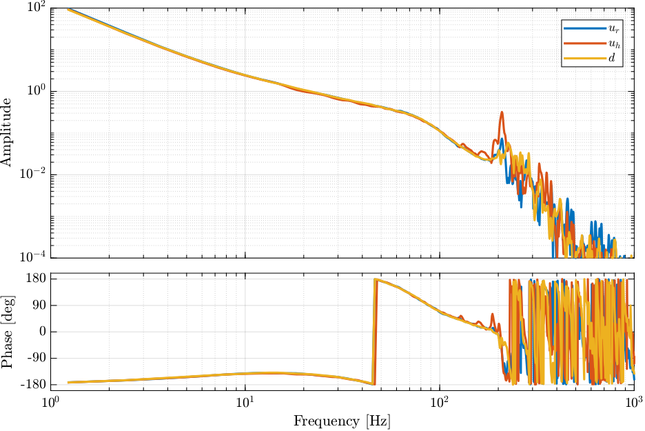
Figure 5: Loop gain
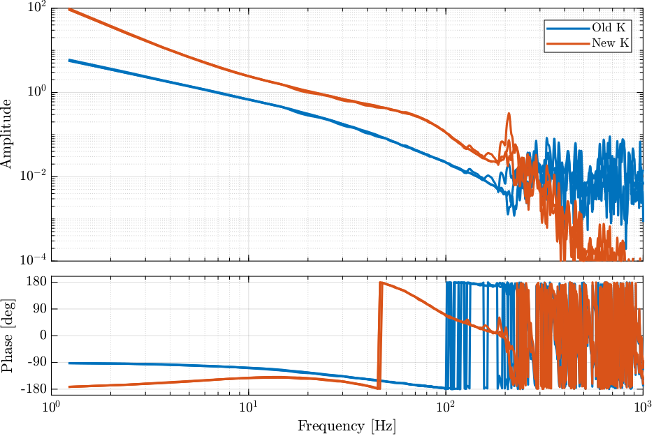
Figure 6: Loop gain
Compare Sensitivity functions
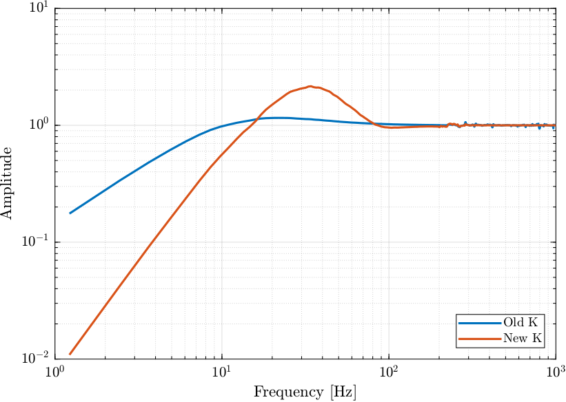
Figure 7: Comparison of sensitivity functions
L  = zeros(3, 3, length(f));
Lb = zeros(3, 3, length(f));

for i_f = 1:length(f)
    L(:,:,i_f)  = [G_ur(i_f,:); G_uh(i_f,:); G_d(i_f,:)]*freqresp(K , f(i_f), 'Hz');
    Lb(:,:,i_f) = [G_ur(i_f,:); G_uh(i_f,:); G_d(i_f,:)]*freqresp(Kb, f(i_f), 'Hz');
end
Figure 8: Root Locus
2.3. Identification - New
ur = load('FJPUR_step_new.mat');
uh = load('FJPUH_step_new.mat');
d  = load('FJPD_step_new.mat');
| 1 | dz311 |
| 2 | dry311 |
| 3 | drx311 |
| 4 | dz111 |
| 5 | dry111 |
| 6 | drx111 |
| 7 | fjpur |
| 8 | fjpuh |
| 9 | fjpd |
| 10 | bragg |
ur.time = ur.time - ur.time(1);
ur.allValues(:, 1) = ur.allValues(:, 1) - mean(ur.allValues(ur.time<0.1, 1));
ur.allValues(:, 2) = ur.allValues(:, 2) - mean(ur.allValues(ur.time<0.1, 2));
ur.allValues(:, 3) = ur.allValues(:, 3) - mean(ur.allValues(ur.time<0.1, 3));

t_filt = ur.time < 5;

ur.u = ur.allValues(t_filt, 7);
ur.y_111 = [-ur.allValues(t_filt, 1), ur.allValues(t_filt, 2), ur.allValues(t_filt, 3)];
uh.time = uh.time - uh.time(1);
uh.allValues(:, 1) = uh.allValues(:, 1) - mean(uh.allValues(uh.time<0.1, 1));
uh.allValues(:, 2) = uh.allValues(:, 2) - mean(uh.allValues(uh.time<0.1, 2));
uh.allValues(:, 3) = uh.allValues(:, 3) - mean(uh.allValues(uh.time<0.1, 3));

uh.u = uh.allValues(t_filt, 8);
uh.y_111 = [-uh.allValues(t_filt, 1), uh.allValues(t_filt, 2), uh.allValues(t_filt, 3)];
d.time = d.time - d.time(1);
d.allValues(:, 1) = d.allValues(:, 1) - mean(d.allValues(d.time<0.1, 1));
d.allValues(:, 2) = d.allValues(:, 2) - mean(d.allValues(d.time<0.1, 2));
d.allValues(:, 3) = d.allValues(:, 3) - mean(d.allValues(d.time<0.1, 3));

d.u = d.allValues(t_filt, 9);
d.y_111 = [-d.allValues(t_filt, 1), d.allValues(t_filt, 2), d.allValues(t_filt, 3)];
J_a_111 = [1,  0.14, -0.0675
           1,  0.14,  0.1525
           1, -0.14,  0.0425];

J_a_311 = [1,  0.14, -0.1525
           1,  0.14,  0.0675
           1, -0.14, -0.0425];

ur.y = [J_a_311 * ur.y_111']';
uh.y = [J_a_311 * uh.y_111']';
d.y  = [J_a_311 * d.y_111']';
%% Sampling Time and Frequency
Ts = 1e-4; % [s]
Fs = 1/Ts; % [Hz]

% Hannning Windows
win = hanning(ceil(5*Fs));
%% And we get the frequency vector
[G_ur, f] = tfestimate(ur.u, ur.y, win, [], [], 1/Ts);
[G_uh, ~] = tfestimate(uh.u, uh.y, win, [], [], 1/Ts);
[G_d,  ~] = tfestimate(d.u,  d.y,  win, [], [], 1/Ts);
[coh_ur, ~] = mscohere(ur.u, ur.y, win, [], [], 1/Ts);
[coh_uh, ~] = mscohere(uh.u, uh.y, win, [], [], 1/Ts);
[coh_d,  ~] = mscohere(d.u,  d.y,  win, [], [], 1/Ts);
%% Previously used controller
load('X_tal_cage_PID.mat', 'K');
%% Controller design
s = tf('s');

% Lead
a  = 4;  % Amount of phase lead / width of the phase lead / high frequency gain
wc = 2*pi*20; % Frequency with the maximum phase lead [rad/s]

% Low Pass Filter
w0 = 2*pi*100; % Cut-off frequency [rad/s]
xi = 0.4; % Damping Ratio

Kb = eye(3)*(2*pi*20)^2/(s^2) *1/(sqrt(a))* (1 + s/(wc/sqrt(a)))/(1 + s/(wc*sqrt(a))) * 1/(1 + 2*xi/w0*s + s^2/w0^2);;
Compare Sensitivity functions
Figure 9: Comparison of sensitivity functions
L  = zeros(3, 3, length(f));
Lb = zeros(3, 3, length(f));

for i_f = 1:length(f)
    L(:,:,i_f)  = [G_ur(i_f,:); G_uh(i_f,:); G_d(i_f,:)]*freqresp(K , f(i_f), 'Hz');
    Lb(:,:,i_f) = [G_ur(i_f,:); G_uh(i_f,:); G_d(i_f,:)]*freqresp(Kb, f(i_f), 'Hz');
end
Figure 10: Root Locus
2.4. Identification - White noise
ur = load('fjpur_white_noise.mat');
uh = load('fjpuh_white_noise.mat');
d  = load('fjpd_white_noise.mat');
| 1 | dz111 |
| 2 | dry111 |
| 3 | drx111 |
| 4 | fjpur |
| 5 | fjpuh |
| 6 | fjpd |
| 7 | bragg |
ur.time = ur.time - ur.time(1);

ur.drx = ur.drx - mean(ur.drx);
ur.dry = ur.dry - mean(ur.dry);
ur.dz  = ur.dz  - mean(ur.dz);
uh.time = uh.time - uh.time(1);

uh.drx = uh.drx - mean(uh.drx);
uh.dry = uh.dry - mean(uh.dry);
uh.dz  = uh.dz  - mean(uh.dz);
d.time = d.time - d.time(1);

d.drx = d.drx - mean(d.drx);
d.dry = d.dry - mean(d.dry);
d.dz  = d.dz  - mean(d.dz);
J_a_111 = [1,  0.14, -0.0675
           1,  0.14,  0.1525
           1, -0.14,  0.0425];

ur.y = [J_a_111 * [-ur.dz, ur.dry, ur.drx]']';
uh.y = [J_a_111 * [-uh.dz, uh.dry, uh.drx]']';
d.y  = [J_a_111 * [-d.dz, d.dry, d.drx]']';
%% Sampling Time and Frequency
Ts = 1e-4; % [s]
Fs = 1/Ts; % [Hz]

% Hannning Windows
win = hanning(ceil(0.5*Fs));
%% And we get the frequency vector
[G_ur, f] = tfestimate(ur.fjpur, ur.y, win, [], [], 1/Ts);
[G_uh, ~] = tfestimate(uh.fjpuh, uh.y, win, [], [], 1/Ts);
[G_d,  ~] = tfestimate(d.fjpd,   d.y,  win, [], [], 1/Ts);
[coh_ur, ~] = mscohere(ur.fjpur, ur.y, win, [], [], 1/Ts);
[coh_uh, ~] = mscohere(uh.fjpuh, uh.y, win, [], [], 1/Ts);
[coh_d,  ~] = mscohere(d.fjpd,   d.y,  win, [], [], 1/Ts);
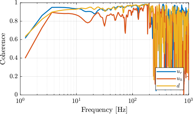
Figure 11: description
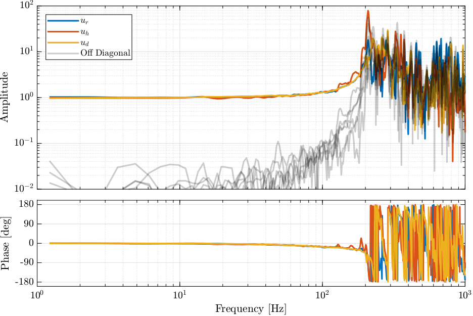
Figure 12: Bode Plot of the DCM dynamics in the frame of the fast jack.
%% Previously used controller
load('X_tal_cage_PID.mat', 'K');
%% Controller design
s = tf('s');

% Lead
a  = 8;  % Amount of phase lead / width of the phase lead / high frequency gain
wc = 2*pi*20; % Frequency with the maximum phase lead [rad/s]

% Low Pass Filter
w0 = 2*pi*80; % Cut-off frequency [rad/s]
xi = 0.4; % Damping Ratio

Kb = eye(3)*(2*pi*20)^2/(s^2) *1/(sqrt(a))* (1 + s/(wc/sqrt(a)))/(1 + s/(wc*sqrt(a))) * 1/(1 + 2*xi/w0*s + s^2/w0^2);;
Figure 13: Loop gain
Figure 14: Loop gain
Compare Sensitivity functions
Figure 15: Comparison of sensitivity functions
L  = zeros(3, 3, length(f));
Lb = zeros(3, 3, length(f));

for i_f = 1:length(f)
    L(:,:,i_f)  = [G_ur(i_f,:); G_uh(i_f,:); G_d(i_f,:)]*freqresp(K , f(i_f), 'Hz');
    Lb(:,:,i_f) = [G_ur(i_f,:); G_uh(i_f,:); G_d(i_f,:)]*freqresp(Kb, f(i_f), 'Hz');
end
Figure 16: Root Locus
2.5. Test
%% Notch
gm = 0.015;
xi = 0.1;
wn = 2*pi*208;

K_notch = (s^2 + 2*gm*xi*wn*s + wn^2)/(s^2 + 2*xi*wn*s + wn^2);
%% Double integrator
w0 = 2*pi*40;
K_int = (w0^2)/(s^2);
%% Lead
a = 3;  % Amount of phase lead / width of the phase lead / high frequency gain
K_lead = 1/(sqrt(a))*(1 + s/(w0/sqrt(a)))/(1 + s/(w0*sqrt(a)));
K_lead = K_lead*K_lead;
%% Low Pass Filter
w0 = 2*pi*120; % Cut-off frequency [rad/s]
xi = 0.3; % Damping Ratio

K_lpf = 1/(1 + 2*xi/w0*s + s^2/w0^2);
%% Diagonal controller
Kb =  0.8*eye(3)*K_notch*K_int*K_lead*K_lpf;
2.6. New controller - Higher bandwidth
%% Previously used controller
load('X_tal_cage_PID.mat', 'K');
%% Current Controller design
% Lead
a  = 8;  % Amount of phase lead / width of the phase lead / high frequency gain
wc = 2*pi*20; % Frequency with the maximum phase lead [rad/s]

% Low Pass Filter
w0 = 2*pi*80; % Cut-off frequency [rad/s]
xi = 0.4; % Damping Ratio

Kb_old = eye(3)*(2*pi*20)^2/(s^2) *1/(sqrt(a))* (1 + s/(wc/sqrt(a)))/(1 + s/(wc*sqrt(a))) * 1/(1 + 2*xi/w0*s + s^2/w0^2);;
%% Notch
gm = 0.015;
xi = 0.2;
wn = 2*pi*208;

K_notch = (s^2 + 2*gm*xi*wn*s + wn^2)/(s^2 + 2*xi*wn*s + wn^2);
%% Double integrator
w0 = 2*pi*40;
K_int = (w0^2)/(s^2);
%% Lead
a = 3;  % Amount of phase lead / width of the phase lead / high frequency gain
w0 = 2*pi*40;
K_lead = 1/(sqrt(a))*(1 + s/(w0/sqrt(a)))/(1 + s/(w0*sqrt(a)));
K_lead = K_lead*K_lead;
%% Low Pass Filter
w0 = 2*pi*120; % Cut-off frequency [rad/s]
xi = 0.3; % Damping Ratio

K_lpf = 1/(1 + 2*xi/w0*s + s^2/w0^2);
%% Diagonal controller
Kb =  0.9*eye(3)*K_notch*K_int*K_lead*K_lpf;
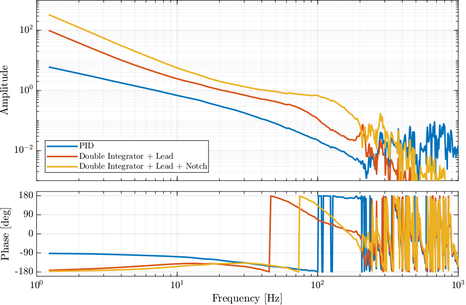
Figure 17: description
L  = zeros(3, 3, length(f));
Lb = zeros(3, 3, length(f));
Lb_new = zeros(3, 3, length(f));

for i_f = 1:length(f)
    L(:,:,i_f)  = [G_ur(i_f,:); G_uh(i_f,:); G_d(i_f,:)]*freqresp(K , f(i_f), 'Hz');
    Lb(:,:,i_f) = [G_ur(i_f,:); G_uh(i_f,:); G_d(i_f,:)]*freqresp(Kb_old, f(i_f), 'Hz');
    Lb_new(:,:,i_f) = [G_ur(i_f,:); G_uh(i_f,:); G_d(i_f,:)]*freqresp(Kb, f(i_f), 'Hz');
end
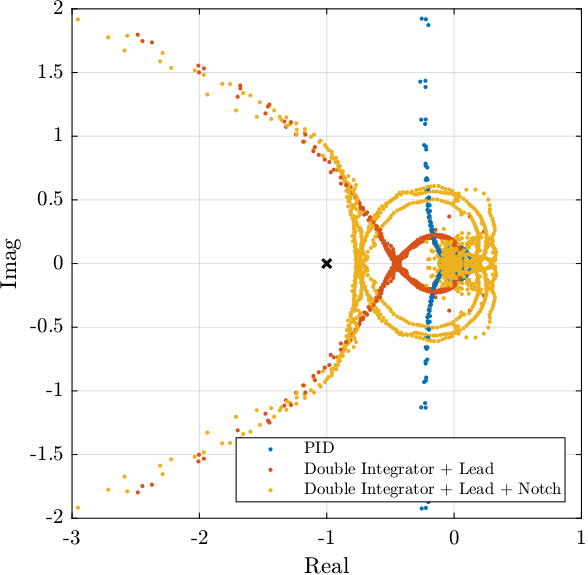
Figure 18: Nyquist Plot
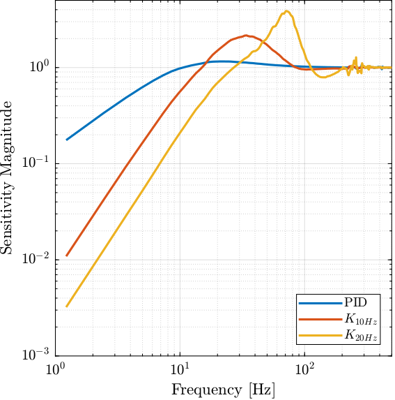
Figure 19: description
2.7. Added gain
%% Notch
gm = 0.015;
xi = 0.2;
wn = 2*pi*208;

K_notch = (s^2 + 2*gm*xi*wn*s + wn^2)/(s^2 + 2*xi*wn*s + wn^2);
%% Double integrator
w0 = 2*pi*40;
K_int = (w0^2)/(s^2);
%% Lead
a = 3;  % Amount of phase lead / width of the phase lead / high frequency gain
w0 = 2*pi*40;
K_lead = 1/(sqrt(a))*(1 + s/(w0/sqrt(a)))/(1 + s/(w0*sqrt(a)));
K_lead = K_lead*K_lead;
%% Low Pass Filter
w0 = 2*pi*120; % Cut-off frequency [rad/s]
xi = 0.3; % Damping Ratio

K_lpf = 1/(1 + 2*xi/w0*s + s^2/w0^2);
gm = 10;
xi = 0.02;
wn = 2*pi*15;

H = (s^2 + 2*gm*xi*wn*s + wn^2)/(s^2 + 2*xi*wn*s + wn^2);
%% Diagonal controller
Kb_gain =  0.9*eye(3)*H*K_notch*K_int*K_lead*K_lpf;
Lb_gain = zeros(3, 3, length(f));

for i_f = 1:length(f)
    Lb_gain(:,:,i_f) = [G_ur(i_f,:); G_uh(i_f,:); G_d(i_f,:)]*freqresp(Kb_gain, f(i_f), 'Hz');
end
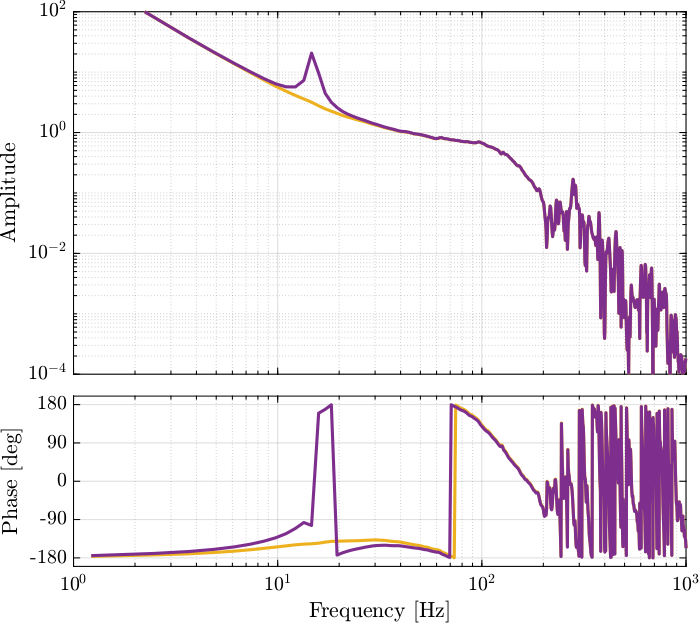
Figure 20: description
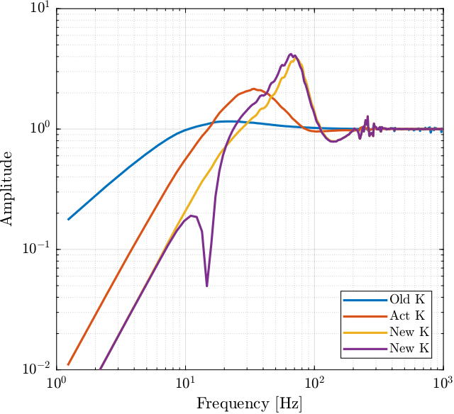
Figure 21: description
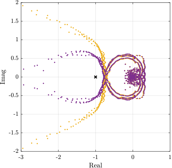
Figure 22: nyquist plot
3. Noise Budgeting
3.1. No Displacement
| 1 | dz311 |
| 2 | dry311 |
| 3 | drx311 |
| 4 | dz111 |
| 5 | dry111 |
| 6 | drx111 |
| 7 | fjpur |
| 8 | fjpuh |
| 9 | fjpd |
| 10 | bragg |
data_10_deg = load('no_mov_10.mat');
data_70_deg = load('no_mov_70.mat');
data_10_deg = extractDatData('no_mov_10.mat', ...
                             {"dz311", "dry311", "drx311", "dz", "dry", "drx", "fjpur", "fjpuh", "fjpd", "bragg"}, ...
                             [1e-9, 1e-9, 1e-9, 1e-9, 1e-9, 1e-9, 1e-8, 1e-8, 1e-8, pi/180]);
data_10_deg = processMeasData(data_10_deg);
Ts = 1e-4;
t = Ts*[1:length(data_10_deg.bragg)];
data_10_deg.dz  = data_10_deg.allValues(:,4) - mean(data_10_deg.allValues(:,4));
data_10_deg.dry = data_10_deg.allValues(:,5) - mean(data_10_deg.allValues(:,5));
data_10_deg.drx = data_10_deg.allValues(:,6) - mean(data_10_deg.allValues(:,6));
%% Compute motion error in the frame of the fast jack
J_a_111 = [1,  0.14, -0.1525
           1,  0.14,  0.0675
           1, -0.14,  0.0425];

de_111 = [data_10_deg.dz'; data_10_deg.dry'; data_10_deg.drx'];
de_fj = J_a_111*de_111;
data_10_deg.fj_ur = de_fj(1,:)';
data_10_deg.fj_uh = de_fj(2,:)';
data_10_deg.fj_d  = de_fj(3,:)';

de_111 = [data_70_deg.dz'; data_70_deg.dry'; data_70_deg.drx'];
de_fj = J_a_111*de_111;
data_70_deg.fj_ur = de_fj(1,:)';
data_70_deg.fj_uh = de_fj(2,:)';
data_70_deg.fj_d  = de_fj(3,:)';
win = hanning(ceil(1/Ts));

[pxx_10_ur, f] = pwelch(data_10_deg.fj_ur, win, [], [], 1/Ts);
[pxx_70_ur, ~] = pwelch(data_70_deg.fj_ur, win, [], [], 1/Ts);

[pxx_10_uh, ~] = pwelch(data_10_deg.fj_uh, win, [], [], 1/Ts);
[pxx_70_uh, ~] = pwelch(data_70_deg.fj_uh, win, [], [], 1/Ts);

[pxx_10_d,  ~] = pwelch(data_10_deg.fj_d,  win, [], [], 1/Ts);
[pxx_70_d,  ~] = pwelch(data_70_deg.fj_d,  win, [], [], 1/Ts);
CPS_10_ur = flip(-cumtrapz(flip(f), flip(pxx_10_ur)));
CPS_10_uh = flip(-cumtrapz(flip(f), flip(pxx_10_uh)));
CPS_10_d  = flip(-cumtrapz(flip(f), flip(pxx_10_d)));

CPS_70_ur = flip(-cumtrapz(flip(f), flip(pxx_70_ur)));
CPS_70_uh = flip(-cumtrapz(flip(f), flip(pxx_70_uh)));
CPS_70_d  = flip(-cumtrapz(flip(f), flip(pxx_70_d)));
figure;
hold on;
plot(f, sqrt(CPS_10_ur), '-' , 'color', colors(1, :), 'DisplayName', '10 deg - $u_r$')
plot(f, sqrt(CPS_70_ur), '--', 'color', colors(1, :), 'DisplayName', '70 deg - $u_r$')
plot(f, sqrt(CPS_10_uh), '-' , 'color', colors(2, :), 'DisplayName', '10 deg - $u_h$')
plot(f, sqrt(CPS_70_uh), '--', 'color', colors(2, :), 'DisplayName', '70 deg - $u_h$')
plot(f, sqrt(CPS_10_d),  '-' , 'color', colors(3, :), 'DisplayName', '10 deg - $d$')
plot(f, sqrt(CPS_70_d),  '--', 'color', colors(3, :), 'DisplayName', '70 deg - $d$')
hold off;
set(gca, 'XScale', 'log'); set(gca, 'YScale', 'log');
xlabel('Frequency [Hz]'); ylabel('ASD [$\frac{nrad}{\sqrt{Hz}}$]');
legend('location', 'northwest');
xlim([1, 1e3]);
figure;
hold on;
plot(f, sqrt(pxx_10_ur))
plot(f, sqrt(pxx_70_ur))
hold off;
set(gca, 'XScale', 'log'); set(gca, 'YScale', 'log');
xlabel('Frequency [Hz]'); ylabel('ASD [$\frac{nrad}{\sqrt{Hz}}$]');
legend('location', 'northwest');
xlim([1, 1e3]);
data_70_deg.dz  = data_70_deg.allValues(:,4) - mean(data_70_deg.allValues(:,4));
data_70_deg.dry = data_70_deg.allValues(:,5) - mean(data_70_deg.allValues(:,5));
data_70_deg.drx = data_70_deg.allValues(:,6) - mean(data_70_deg.allValues(:,6));
win = hanning(ceil(1/Ts));

[pxx_10_drx, f] = pwelch(data_10_deg.drx, win, [], [], 1/Ts);
[pxx_70_drx, ~] = pwelch(data_70_deg.drx, win, [], [], 1/Ts);

[pxx_10_dry, ~] = pwelch(data_10_deg.dry, win, [], [], 1/Ts);
[pxx_70_dry, ~] = pwelch(data_70_deg.dry, win, [], [], 1/Ts);

[pxx_10_dz,  ~] = pwelch(data_10_deg.dz,  win, [], [], 1/Ts);
[pxx_70_dz,  ~] = pwelch(data_70_deg.dz,  win, [], [], 1/Ts);
figure;
hold on;
plot(f, sqrt(pxx_10_drx))
plot(f, sqrt(pxx_70_drx))
hold off;
set(gca, 'XScale', 'log'); set(gca, 'YScale', 'log');
xlabel('Frequency [Hz]'); ylabel('ASD [$\frac{nrad}{\sqrt{Hz}}$]');
legend('location', 'northwest');
xlim([1, 1e3]);
figure;
hold on;
plot(f, sqrt(pxx_10_dry))
plot(f, sqrt(pxx_70_dry))
hold off;
set(gca, 'XScale', 'log'); set(gca, 'YScale', 'log');
xlabel('Frequency [Hz]'); ylabel('ASD [$\frac{nrad}{\sqrt{Hz}}$]');
legend('location', 'northwest');
xlim([1, 1e3]);
figure;
hold on;
plot(f, sqrt(pxx_10_dz))
plot(f, sqrt(pxx_70_dz))
hold off;
set(gca, 'XScale', 'log'); set(gca, 'YScale', 'log');
xlabel('Frequency [Hz]'); ylabel('ASD [$\frac{nm}{\sqrt{Hz}}$]');
legend('location', 'northwest');
xlim([1, 1e3]);
3.2. Scans
| 1 | dz311 |
| 2 | dry311 |
| 3 | drx311 |
| 4 | dz111 |
| 5 | dry111 |
| 6 | drx111 |
| 7 | fjpur |
| 8 | fjpuh |
| 9 | fjpd |
| 10 | bragg |
%% Load Data
data_10_70_deg = extractDatData('thtraj_10_70.mat', ...
                             {"dz311", "dry311", "drx311", "dz", "dry", "drx", "fjur", "fjuh", "fjd", "bragg"}, ...
                             [1e-9, 1e-9, 1e-9, 1e-9, 1e-9, 1e-9, 1e-8, 1e-8, 1e-8, pi/180]);

Ts = 1e-4;
t = Ts*[1:length(data_10_70_deg.bragg)];

%% Actuator Jacobian
J_a_111 = [1,  0.14, -0.0675
           1,  0.14,  0.1525
           1, -0.14,  0.0425];

data_10_70_deg.ddz  = 10.5e-3./(2*cos(data_10_70_deg.bragg)) - data_10_70_deg.dz;

%% Computation of the position of the FJ as measured by the interferometers
error = J_a_111 * [data_10_70_deg.ddz, data_10_70_deg.dry, data_10_70_deg.drx]';

data_10_70_deg.fjur_e = error(1,:)'; % [m]
data_10_70_deg.fjuh_e = error(2,:)'; % [m]
data_10_70_deg.fjd_e  = error(3,:)'; % [m]
%% Load Data
data_70_10_deg = extractDatData('thtraj_70_10.mat', ...
                             {"dz311", "dry311", "drx311", "dz", "dry", "drx", "fjur", "fjuh", "fjd", "bragg"}, ...
                             [1e-9, 1e-9, 1e-9, 1e-9, 1e-9, 1e-9, 1e-8, 1e-8, 1e-8, pi/180]);
%% Actuator Jacobian
J_a_111 = [1,  0.14, -0.0675
           1,  0.14,  0.1525
           1, -0.14,  0.0425];

data_70_10_deg.ddz  = 10.5e-3./(2*cos(data_70_10_deg.bragg)) - data_70_10_deg.dz;

%% Computation of the position of the FJ as measured by the interferometers
error = J_a_111 * [data_70_10_deg.ddz, data_70_10_deg.dry, data_70_10_deg.drx]';

data_70_10_deg.fjur_e = error(1,:)'; % [m]
data_70_10_deg.fjuh_e = error(2,:)'; % [m]
data_70_10_deg.fjd_e  = error(3,:)'; % [m]
win = hanning(ceil(1/Ts));

[pxx_10_70_ur, f] = pwelch(data_10_70_deg.fjur_e(t<100), win, [], [], 1/Ts);
[pxx_70_10_ur, ~] = pwelch(data_70_10_deg.fjur_e(t<100), win, [], [], 1/Ts);

[pxx_10_70_uh, ~] = pwelch(data_10_70_deg.fjuh_e(t<100), win, [], [], 1/Ts);
[pxx_70_10_uh, ~] = pwelch(data_70_10_deg.fjuh_e(t<100), win, [], [], 1/Ts);

[pxx_10_70_d,  ~] = pwelch(data_10_70_deg.fjd_e(t<100),  win, [], [], 1/Ts);
[pxx_70_10_d,  ~] = pwelch(data_70_10_deg.fjd_e(t<100),  win, [], [], 1/Ts);
CPS_10_70_ur = flip(-cumtrapz(flip(f), flip(pxx_10_70_ur)));
CPS_10_70_uh = flip(-cumtrapz(flip(f), flip(pxx_10_70_uh)));
CPS_10_70_d  = flip(-cumtrapz(flip(f), flip(pxx_10_70_d)));

CPS_70_10_ur = flip(-cumtrapz(flip(f), flip(pxx_70_10_ur)));
CPS_70_10_uh = flip(-cumtrapz(flip(f), flip(pxx_70_10_uh)));
CPS_70_10_d  = flip(-cumtrapz(flip(f), flip(pxx_70_10_d)));
figure;
hold on;
plot(f, 1e9*sqrt(CPS_10_70_ur))
hold off;
set(gca, 'XScale', 'log'); set(gca, 'YScale', 'log');
xlabel('Frequency [Hz]'); ylabel('ASD [$\frac{nrad}{\sqrt{Hz}}$]');
legend('location', 'northwest');
xlim([1, 1e3]);
figure;
hold on;
plot(f, sqrt(pxx_10_70_ur))
plot(f, sqrt(pxx_70_10_ur))
hold off;
set(gca, 'XScale', 'log'); set(gca, 'YScale', 'log');
xlabel('Frequency [Hz]'); ylabel('ASD [$\frac{nrad}{\sqrt{Hz}}$]');
legend('location', 'northwest');
xlim([1, 1e3]);
3.3. Noise budgeting - No rotation
First, we look at the position errors when the bragg axis is not moving
%% Load Measurement Data
ol_data = load('FJPUR_step.mat');
%% Pre-processing
ol_time = ol_data.time - ol_data.time(1);

ol_drx = ol_data.allValues(ol_time < 45, 6);
ol_dry = ol_data.allValues(ol_time < 45, 5);
ol_dz  = ol_data.allValues(ol_time < 45, 4);

ol_drx = ol_drx - mean(ol_drx);
ol_dry = ol_dry - mean(ol_dry);
ol_dz = ol_dz - mean(ol_dz);

ol_time = ol_time(ol_time < 45);
figure;
plot(ol_time, ol_drx)
%% Parameters for Spectral Analysis
Ts = 1e-4;
win = hanning(ceil(1/Ts));
%% Computation of the PSD
[pxx_ol_drx, f] = pwelch(ol_drx, win, [], [], 1/Ts);
[pxx_ol_dry, ~] = pwelch(ol_dry, win, [], [], 1/Ts);
[pxx_ol_dz,  ~] = pwelch(ol_dz,  win, [], [], 1/Ts);
Figure 23: Amplitude Spectral Density
%% Cumulative Spectral Density
CPS_drx = flip(-cumtrapz(flip(f), flip(pxx_ol_drx)));
CPS_dry = flip(-cumtrapz(flip(f), flip(pxx_ol_dry)));
CPS_dz  = flip(-cumtrapz(flip(f), flip(pxx_ol_dz)));
%% Cumulative Spectral Density
CPS_drx = cumtrapz(f, pxx_ol_drx);
CPS_dry = cumtrapz(f, pxx_ol_dry);
CPS_dz  = cumtrapz(f, pxx_ol_dz);
Figure 24: Cumulative Amplitude Spectrum
3.4. Noise budgeting - Bragg rotation
4. Test Mode C
4.1. Mode B and Mode C
data_B = extractDatData(sprintf("/home/thomas/mnt/data_id21/22Jan/blc13491/id21/test_regul_220119/%s","lut_const_fj_vel_19012022_1450.dat"), ...
                             {"bragg", "dz", "dry", "drx", "fjur", "fjuh", "fjd"}, ...
                             [pi/180, 1e-9, 1e-9, 1e-9, 1e-8, 1e-8, 1e-8]);
data_B = processMeasData(data_B);
data_C = extractDatData(sprintf("/home/thomas/mnt/data_id21/22Jan/blc13491/id21/test_regul_220119/%s","lut_const_fj_vel_19012022_1454.dat"), ...
                             {"bragg", "dz", "dry", "drx", "fjur", "fjuh", "fjd"}, ...
                             [pi/180, 1e-9, 1e-9, 1e-9, 1e-8, 1e-8, 1e-8]);
data_C = processMeasData(data_C);
figure;
hold on;
plot(180/pi*data_B.bragg, 1e9*data_B.drx)
hold off;
xlabel('Bragg Angle [deg]'); ylabel('DRX [nrad]');
figure;
hold on;
plot(180/pi*data_B.bragg, 1e9*data_B.fjur_e_filt)
plot(180/pi*data_C.bragg, 1e9*data_C.fjur_e_filt)
hold off;
xlabel('Bragg Angle [deg]'); ylabel('FJUR Error [nm]');
figure;
hold on;
plot(180/pi*data_B.bragg, 1e9*data_B.fjur_e)
plot(180/pi*data_C.bragg, 1e9*data_C.fjur_e)
hold off;
xlabel('Bragg Angle [deg]'); ylabel('FJUR Error [nm]');
%% FIR Filter
Fs = 1e4; % Sampling Frequency [Hz]
fir_order = 5000; % Filter's order
delay = fir_order/2; % Delay induced by the filter
B_fir = firls(5000, ... % Filter's order
              [0 5/(Fs/2)  10/(Fs/2) 1], ... % Frequencies [Hz]
              [1 1          0        0]); % Wanted Magnitudes
%% Filtering all measured Fast Jack Position using the FIR filter
data_B.drx_filter = filter(B_fir, 1, data_B.drx);
data_B.drx_filter(1:end-delay) = data_B.drx_filter(delay+1:end);

data_C.drx_filter = filter(B_fir, 1, data_C.drx);
data_C.drx_filter(1:end-delay) = data_C.drx_filter(delay+1:end);
figure;
hold on;
plot(180/pi*data_B.bragg, 1e9*data_B.drx_filter)
plot(180/pi*data_C.bragg, 1e9*data_C.drx_filter)
hold off;
xlabel('Bragg Angle [deg]'); ylabel('DRX [nrad]');
Ts = 1e-4;
win = hanning(ceil(1/Ts));

[pxx_B_drx, f] = pwelch(data_B.drx, win, [], [], 1/Ts);
[pxx_C_drx, ~] = pwelch(data_C.drx, win, [], [], 1/Ts);
5. Export numerator and denominator
5.1. Export
K_order = 10;
load('X_tal_cage_PID.mat', 'K');
K_order = order(K(1,1));
Kz = c2d(K(1,1)*(1 + s/2/pi/2e3)^(9-K_order)/(1 + s/2/pi/2e3)^(9-K_order), 1e-4);
[num, den] = tfdata(Kz, 'v');

formatSpec = '%.18e %.18e %.18e %.18e %.18e %.18e %.18e %.18e %.18e %.18e\n';
fileID = fopen('X_tal_cage_PID.dat', 'w');
fprintf(fileID, formatSpec, [num; den]');
fclose(fileID);
load('X_tal_cage_PID_20Hz.mat', 'K');
K_order = order(K(1,1));
Kz = c2d(K(1,1)*(1 + s/2/pi/2e3)^(9-K_order)/(1 + s/2/pi/2e3)^(9-K_order), 1e-4);
[num, den] = tfdata(Kz, 'v');

formatSpec = '%.18e %.18e %.18e %.18e %.18e %.18e %.18e %.18e %.18e %.18e\n';
fileID = fopen('X_tal_cage_PID_20Hz.dat', 'w');
fprintf(fileID, formatSpec, [num; den]');
fclose(fileID);
load('X_tal_cage_PID_40Hz.mat', 'K');
K_order = order(K(1,1));
Kz = c2d(K(1,1)*(1 + s/2/pi/2e3)^(9-K_order)/(1 + s/2/pi/2e3)^(9-K_order), 1e-4);
[num, den] = tfdata(Kz, 'v');

formatSpec = '%.18e %.18e %.18e %.18e %.18e %.18e %.18e %.18e %.18e %.18e\n';
fileID = fopen('X_tal_cage_PID_40Hz.dat', 'w');
fprintf(fileID, formatSpec, [num; den]');
fclose(fileID);
5.2. Verify
K_data = importdata('X_tal_cage_PID_20Hz.dat');
K = tf(K_data(1,:), K_data(2,:), 1e-4)