ESRF Double Crystal Monochromator - Bragg Control

1. Architecture
2. Current Loop
3. Position Feedback Loop
4. Velocity Feedback Loop
5. Feedforward Controller

This report is also available as a pdf.

1. Architecture

1.1. Hardware

A schematic of the hardware involved in the control of the bragg angle is shown in Figure 2.

The IcePAP is used to generated the reference signal (i.e. requested Bragg angle) which is sent to the Aerotech using 32bits digital numbers. The IcePAP can be configured and motions can be triggered from BLISS.

The Aerotech job is to control the Bragg angle from encoder measurement (averaged by the PEPU). It can be configured using some Aerotech software from a Windows computer.

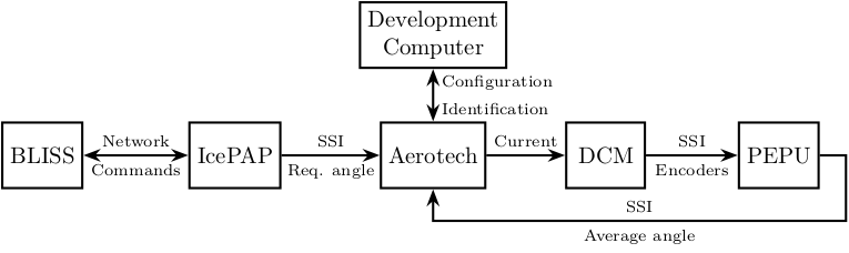
Figure 1: Hardware involved in the Bragg control

1.2. Software

Two software are used:

Ensemble Configuration Manager: to access and change configuration
Ensemble Digital Scope: to identify the dynamics and tune the controllers

1.2.1. Ensemble Configuration Manager

Click on DCM and then connect. Right click and Parameters and then Retreive Parameters. Interesting parameters can be found in:

Axis/Current Loop: parameters of the current loop
Axis/Servo Loop: general parameters for the servo loop, especially the sampling rate
Axis/Servo Loop/Gains: all gains for controllers
Axis/Servo Loop/Filters: additional filters to be used
Axis/Fault/Thresholds: used to set safety values

In Tools/Other Calculators/Digital Filter Calculator easy computation of filter coefficients can be done.

To save parameters, right click on DCM and then Save Parameters to.... The parameters will be saved to a .prme text file.

1.2.2. Ensemble Digital Scope

For system identification:

Click on the Loop Transmission tab
In the menu Configuration / Control Loop select Current Loop or Servo Loop
Choose the excitation signal in menu Configuration / Input Type
Choose which value to measure and which signal to excite in menu Configuration / Response Type
Then choose the identification parameters:
- Start Freq [Hz]
- End Freq [Hz]
- # Division
- % Max Current can be set to 2% to start

To display and save signals:

Click on the Scope tab
In the Configuration menu, choose the number of points and the sampling time
The signals to be saved can be configured using menu Configuration / Configure Data Collection
Then, the data can be displayed by clicking on button Collect One Set of Data
Power Spectral Density of signals can be computed using menu Tool / Fourier Transform
Data can be saved using menu File / Export To
Displacements (ramps) may be performed using the command moveinc X 0.1 F 10. This particular command will trigger a incremental displacement of 0.1 degrees with a velocity of 10 deg/s.

1.2.3. Units

Signals are usually expressed in Counts. Here, one count is defined as one increment of the encoder value. This corresponds to \(2\pi/2^{31} \approx 3\,\text{nrad}\) (\(2^{31}\) encoder values for one turn).

The unit is one degree. There are therefore \(2^{31}/360 \approx 5965232 \text{ count/unit}\).

The time unit taken is the millisecond.

1.3. Control Architecture

The control architecture is schematically shown in Figure 2.

It is composed of several parts that are fixed by the Aerotech hardware and software:

The current loop in yellow which is used to regulate the current sent to the Bragg motor.
The position feedback loop in blue used to regulate the position of the bragg angle based on the encoder
The velocity feedback loop in green that can optionally be added to further control the angular velocity
The feedforward controller in red that can be used to further increase control performances

Each of them containing some controllers with fixed structures (e.g. PID, second order filters, …).

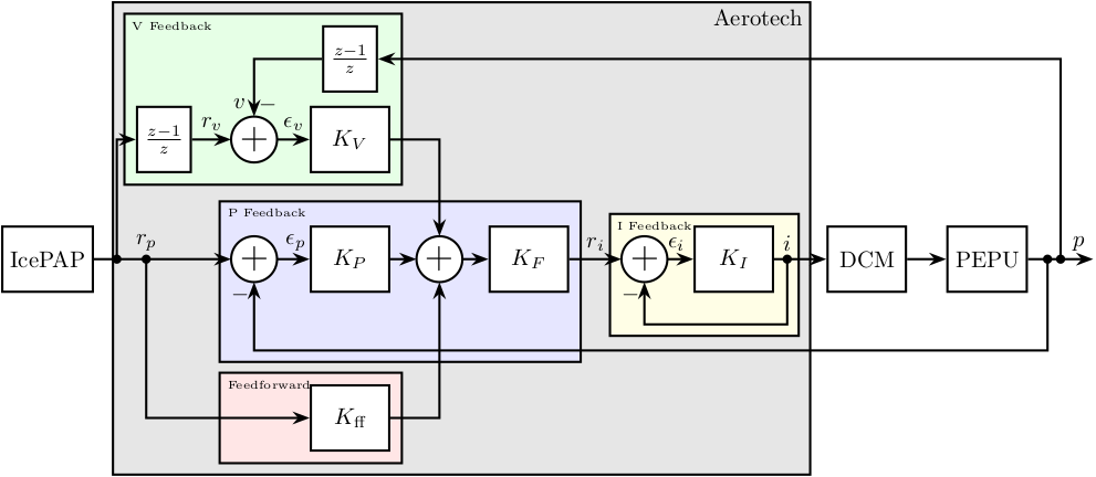
Figure 2: Complete control architecture for Bragg Angle

The requested Bragg angle is generated on the IcePAP while the measured bragg angle is done using encoders and is averaged and converted by the PEPU. Everything inside the grey area in Figure 2 is what is computed inside the Aerotech controller.

2. Current Loop

The first loop is used to control the current sent to the motor.

Its structure is shown in Figure 3. Signals are:

\(r_i\) is the requested current in Amperes
\(i\) is the generated current in Amperes
\(\epsilon_i\) is the errors in current in Amperes
\(p\) the measured Bragg angle

The controller for the current feedback has a fixed structure (PI controller):

\begin{equation} \label{eq:K_current_loop} \boxed{K_I(z) = k_{I,p} + \frac{z+1}{z-1} \cdot k_{I,i}} \end{equation}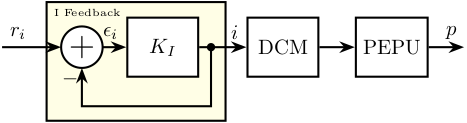

Figure 3: Current Feedback

Therefore, two parameters have to be tuned:

CurrentGainKp the proportional gain (\(k_{I,p}\))
CurrentGainKi the integral gain (\(K_{I,i}\))

In order to properly design the controller:

The system dynamics is identified (Section 2.1)
The two gains are tuned based on the identified dynamics (Section 2.2)
The performances are verified by identifying the dynamics of the closed loop system (Section 2.3)

2.1. Identification

2.2. Controller Design

Table 1: Parameters for the Current Loop Controller
Variable Name	Notation	Initial	Re-tuned
`CurrentGainKp`	\(K_{I,p}\)	60000
`CurrentGainKi`	\(K_{I,i}\)	525

2.3. Performance Verification

3. Position Feedback Loop

A second loop can be closed to control the position of the bragg angle (Figure 4).

The signals are:

\(p\) is the measured angle
\(r_p\) is the requested angle (steps generated by the IcePAP)
\(\epsilon = r_p - p\) is the angle error

The filter \(K_P\) is a PID controller:

\begin{equation} \label{eq:K_servo_loop} \boxed{K_P(z) = k_{P,p} + k_{P,i} \left(\frac{z}{z-1}\right) + k_{P,d} \left(\frac{z-1}{z}\right) } \end{equation}

The filter \(K_F\) can contain up to eight second order digital filters \(K_{F,i}\).

\begin{equation} \label{eq:K_servo_filter} \boxed{K_{F_i}(z) = \frac{N_{i,0} + N_{i,1} z^{-1} + N_{i,2} z^{-2}}{1 + D_{i,1} z^{-1} + D_{i,2} z^{-2}}} \end{equation}

Such filter can represent:

Second order low pass filter
Notch
Lead, Lags, …

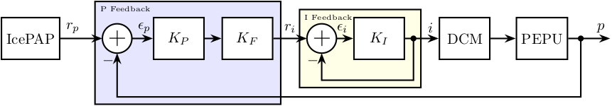
Figure 4: Position Feedback

3.1. Identification

3.2. Controller Design

Table 2: Parameters for the Position Loop Controller
Variable Name	Notation	Initial
`GainKd1`	\(K_{P_d}\)	12800
`GainKp1`	\(K_{P_p}\)	2.4
`GainKpi`	\(K_{P_i}\)	0.32

3.3. Performance Verification

4. Velocity Feedback Loop

An additional Loop may be added which is used to control the angular velocity. Added signals are:

\(v\) the measured velocity (based on encoder information)
\(r_v\) the requested velocity (based on derivation of the requested position)
\(\epsilon_v\) the estimated velocity error

The controller \(K_V\) has a PI structure:

\begin{equation} \label{eq:K_velocity_feedback} \boxed{K_V(z) = k_{V,p} + k_{V,i} \left(\frac{z}{z-1}\right) } \end{equation}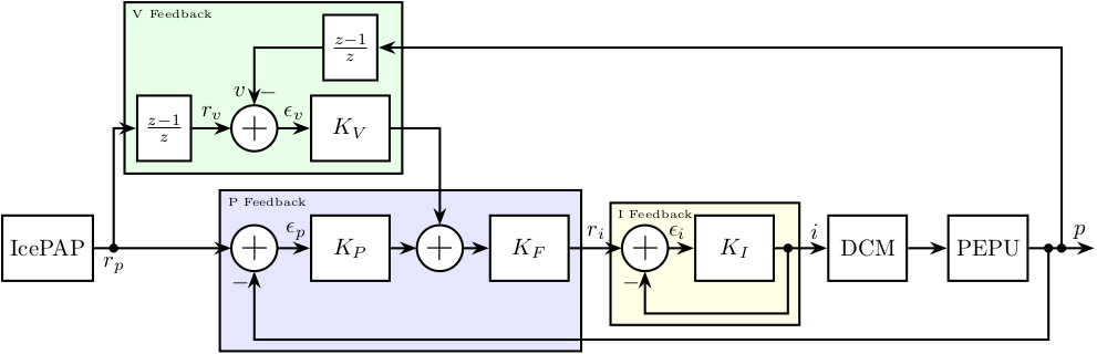

Figure 5: Velocity Feedback Feedback

4.1. Identification

4.2. Controller Design

4.3. Performance Verification

5. Feedforward Controller

Finally, a feedforward controller may be added. This feedforward controller is only based on the requested position (no feedback on the measured position is performed).

The structure of the feedforward controller is:

\begin{equation} \label{eq:K_feedforward} \boxed{K_{\text{ff}}(z) = k_{\text{ff},p} + k_{\text{ff},v} \left(\frac{z-1}{z}\right) + k_{\text{ff},a} \left(\frac{z-1}{z}\right)^2 } \end{equation}

The output of the controller may be added before \(K_F\) (as shown in Figure 6) or after.

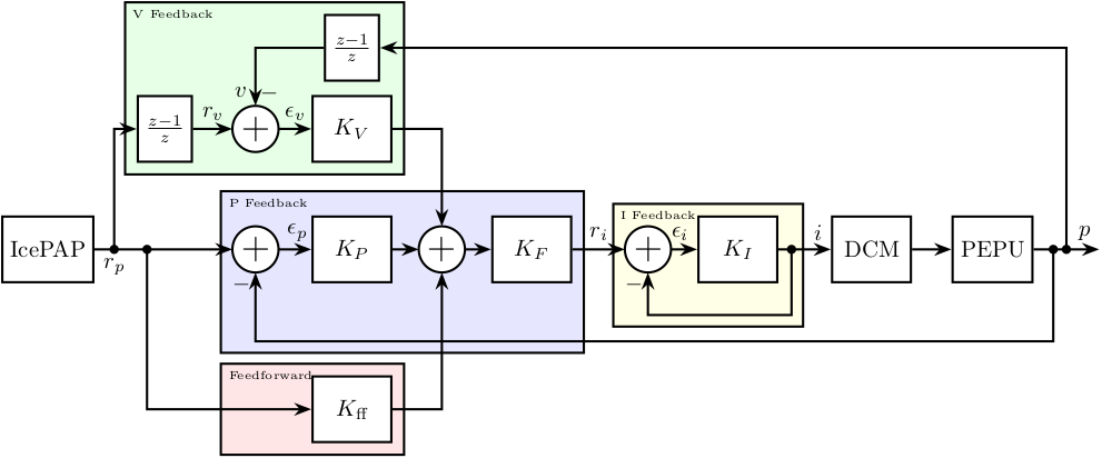
Figure 6: Added Feedforward controller