Attocube - Test Bench
Table of Contents
This report is also available as a pdf.
In this document, few caracteristics of the Attocube Displacement Measuring Interferometer IDS3010 (link) are studied:
- Section 1: the ASD noise of the measured displacement is estimated
- Section 2: the effect of two air protections on the stability of the measurement is studied
- Section 3: the cyclic non-linearity of the attocube is estimated using a encoder
1 Estimation of the Spectral Density of the Attocube Noise
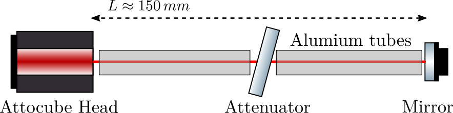
Figure 1: Test Bench Schematic
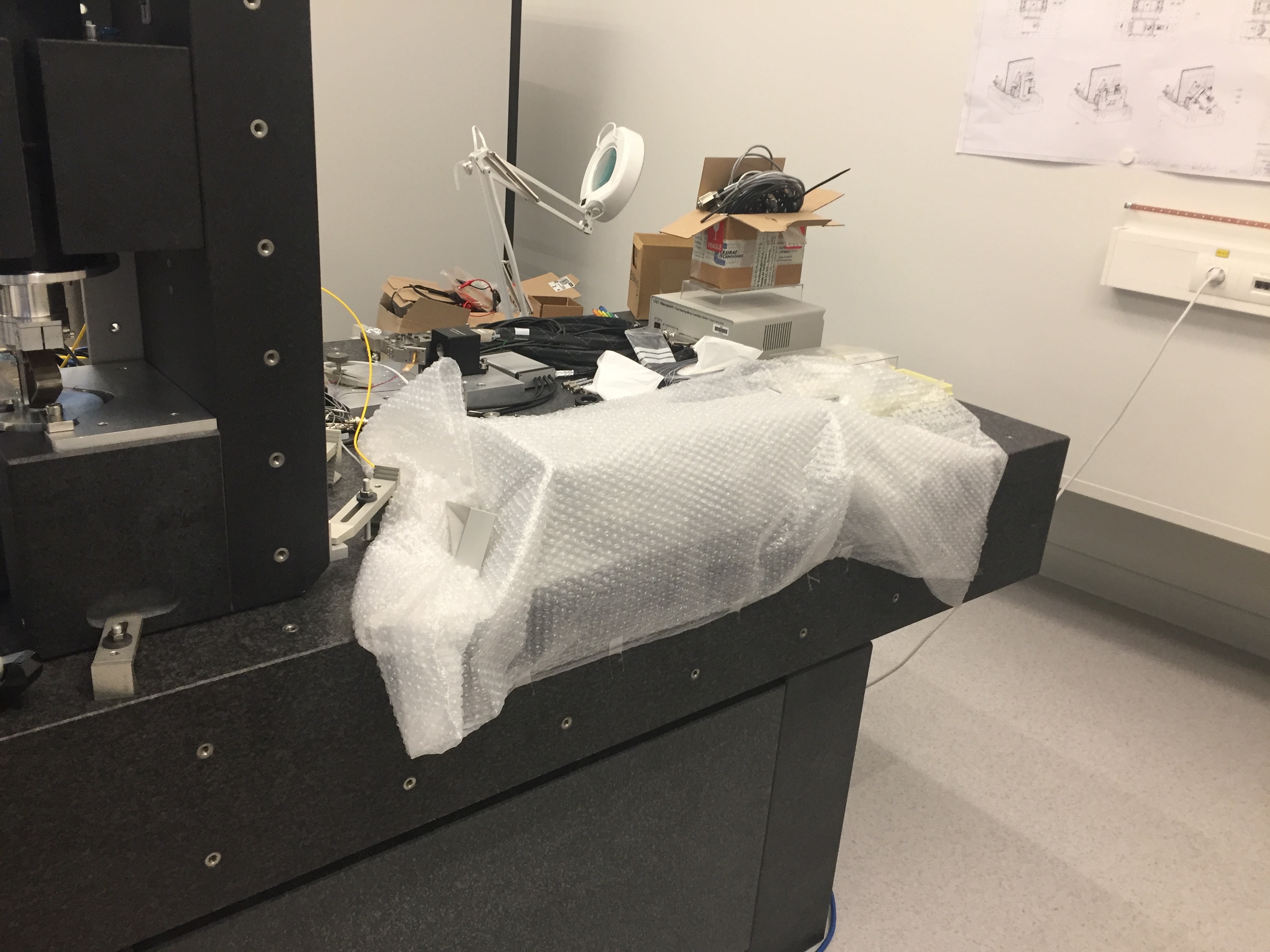
Figure 2: Picture of the test bench. The Attocube and mirror are covered by a “bubble sheet”
1.1 Long and Slow measurement
The first measurement was made during ~17 hours with a sampling time of \(T_s = 0.1\,s\).
  load('long_test_plastic.mat', 'x', 't')
  Ts = 0.1; % [s]
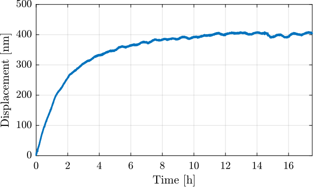
Figure 3: Long measurement time domain data
Let’s fit the data with a step response to a first order low pass filter (Figure 4).
  f = @(b,x) b(1)*(1 - exp(-x/b(2)));

  y_cur = x(t < 17.5*60*60);
  t_cur = t(t < 17.5*60*60);

  nrmrsd = @(b) norm(y_cur - f(b,t_cur)); % Residual Norm Cost Function
  B0 = [400e-9, 2*60*60];                        % Choose Appropriate Initial Estimates
  [B,rnrm] = fminsearch(nrmrsd, B0);     % Estimate Parameters ‘B’
The corresponding time constant is (in [h]):
2.0658
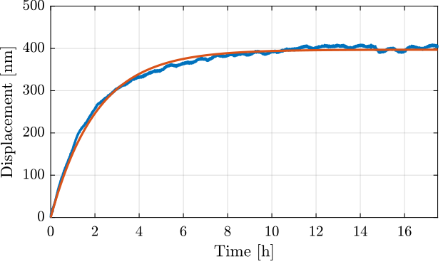
Figure 4: Fit of the measurement data with a step response of a first order low pass filter
We can see in Figure 3 that there is a transient period where the measured displacement experiences some drifts.
This is probably due to thermal effects.
We only select the data between t1 and t2.
The obtained displacement is shown in Figure 5.
  t1 = 10.5; t2 = 17.5; % [h]

  x = x(t > t1*60*60 & t < t2*60*60);
  x = x - mean(x);
  t = t(t > t1*60*60 & t < t2*60*60);
  t = t - t(1);
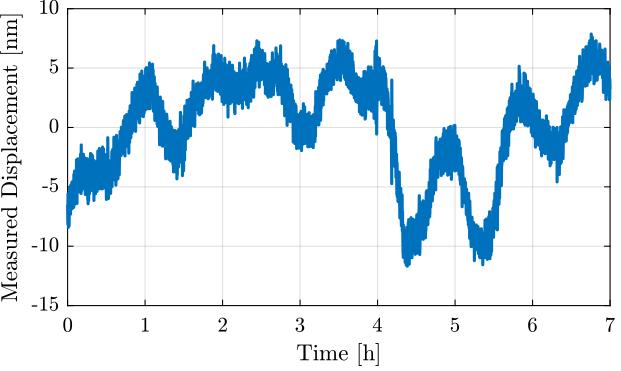
Figure 5: Kept data (removed slow drifts during the first hours)
The Power Spectral Density of the measured displacement is computed
  win = hann(ceil(length(x)/20));
  [p_1, f_1] = pwelch(x, win, [], [], 1/Ts);
As a low pass filter was used in the measurement process, we multiply the PSD by the square of the inverse of the filter’s norm.
  G_lpf = 1/(1 + s/2/pi);
  p_1 = p_1./abs(squeeze(freqresp(G_lpf, f_1, 'Hz'))).^2;
Only frequencies below 2Hz are taken into account (high frequency noise will be measured afterwards).
  p_1 = p_1(f_1 < 2);
  f_1 = f_1(f_1 < 2);
1.2 Short and Fast measurement
An second measurement is done in order to estimate the high frequency noise of the interferometer. The measurement is done with a sampling time of \(T_s = 0.1\,ms\) and a duration of ~100s.
  load('short_test_plastic.mat')
  Ts = 1e-4; % [s]
x = detrend(x, 0);
The time domain measurement is shown in Figure 6.
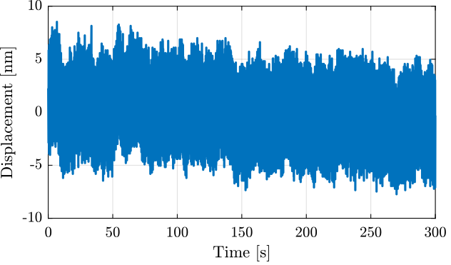
Figure 6: Time domain measurement with the high sampling rate
The Power Spectral Density of the measured displacement is computed
  win = hann(ceil(length(x)/20));
  [p_2, f_2] = pwelch(x, win, [], [], 1/Ts);
1.3 Obtained Amplitude Spectral Density of the measured displacement
The computed ASD of the two measurements are combined in Figure 7.
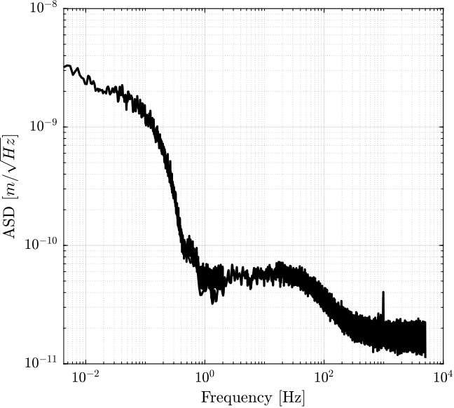
Figure 7: Obtained Amplitude Spectral Density of the measured displacement
2 Effect of the “bubble sheet” and “Aluminium tube”
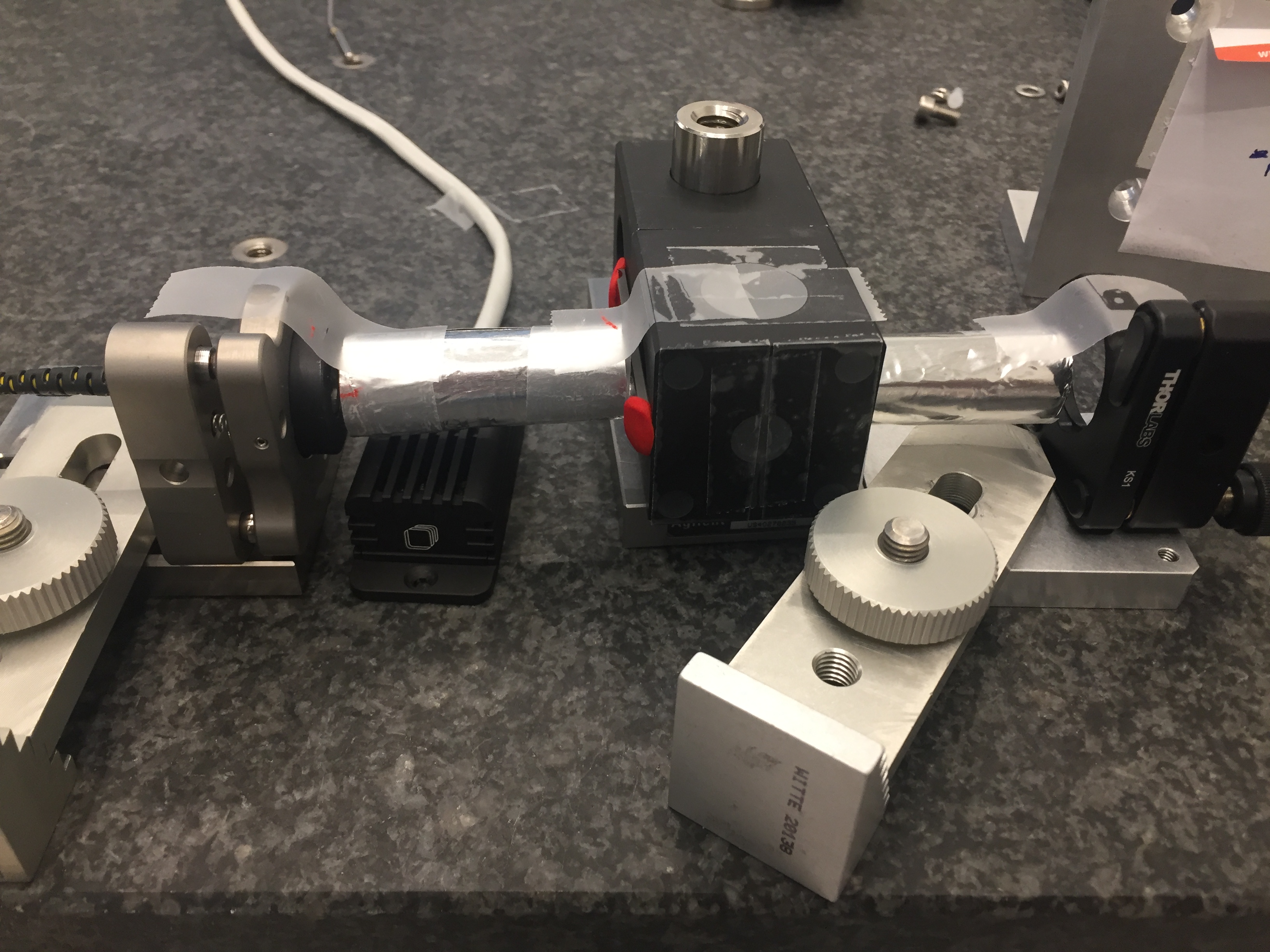
Figure 8: Aluminium tube used to protect the beam path from disturbances
Measurements corresponding to the used of both the aluminium tube and the “bubble sheet ”are loaded and PSD is computed.
  load('short_test_plastic.mat');
  Ts = 1e-4; % [s]

  t_1 = t;
  x_1 = detrend(x, 0);

  [p_1, f_1] = pwelch(x_1, win, [], [], 1/Ts);
Then, the measurement corresponding to the use of the aluminium tube only are loaded and the PSD is computed.
  load('short_test_alu_tube.mat');
  Ts = 1e-4; % [s]

  t_2 = t;
  x_2 = detrend(x, 0);

  [p_2, f_2] = pwelch(x_2, win, [], [], 1/Ts);
Finally, the measurements when neither using the aluminium tube nor the “bubble sheet” are used.
  load('short_test_without_material.mat');
  Ts = 1e-4; % [s]

  t_3 = t;
  x_3 = detrend(x, 0);

  [p_3, f_3] = pwelch(x_3, win, [], [], 1/Ts);
The time domain signals are compared in Figure 9 and the power spectral densities are compared in Figure 10.
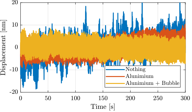
Figure 9: Time domain signals
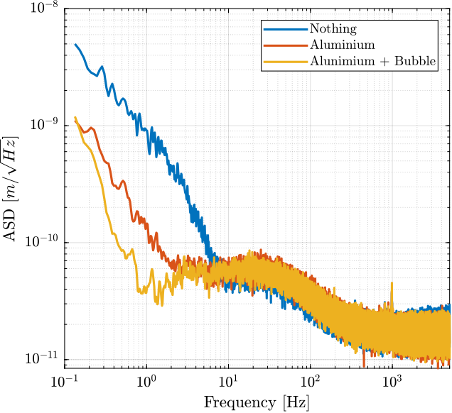
Figure 10: Comparison of the noise ASD with and without bubble sheet
3 Measurement of the Attocube’s non-linearity
The measurement setup is shown in Figure 11.
Here are the equipment used in the test bench:
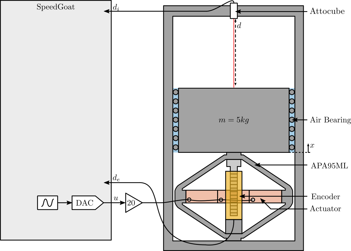
Figure 11: Schematic of the Experiment
A DAC and voltage amplified are used to move the mass with the Amplified Piezoelectric Actuator (APA95ML). The encoder and the attocube are measure ring the same motion.
As will be shown shortly, this measurement permitted to measure the period non-linearity of the Attocube.
3.1 Load Data
The measurement data are loaded and the offset are removed using the detrend command.
  load('int_enc_comp.mat', 'interferometer', 'encoder', 'u', 't');
  Ts = 1e-4; % Sampling Time [s]
  interferometer = detrend(interferometer, 0);
  encoder = detrend(encoder, 0);
  u = detrend(u, 0);
3.2 Time Domain Results
One period of the displacement of the mass as measured by the encoder and interferometer are shown in Figure 12. It consist of the sinusoidal motion at 0.5Hz with an amplitude of approximately \(70\mu m\).
The frequency of the motion is chosen such that no resonance in the system is excited. This should improve the coherence between the measurements made by the encoder and interferometer.
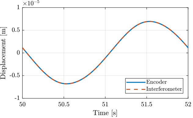
Figure 12: One cycle measurement
The difference between the two measurements during the same period is shown in Figure 13.
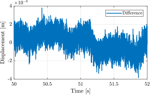
Figure 13: Difference between the Encoder and the interferometer during one cycle
3.3 Difference between Encoder and Interferometer as a function of time
The data is filtered using a second order low pass filter with a cut-off frequency \(\omega_0\) as defined below.
  w0 = 2*pi*5; % [rad/s]
  xi = 0.7;

  G_lpf = 1/(1 + 2*xi/w0*s + s^2/w0^2);
After filtering, the data is “re-shaped” such that we can superimpose all the measured periods as shown in Figure 14. This gives an idea of the measurement error as given by the Attocube during a \(70 \mu m\) motion.
  d_err_mean = reshape(lsim(G_lpf, encoder - interferometer, t), [2/Ts floor(Ts/2*length(encoder))]);
  d_err_mean = d_err_mean - mean(d_err_mean);
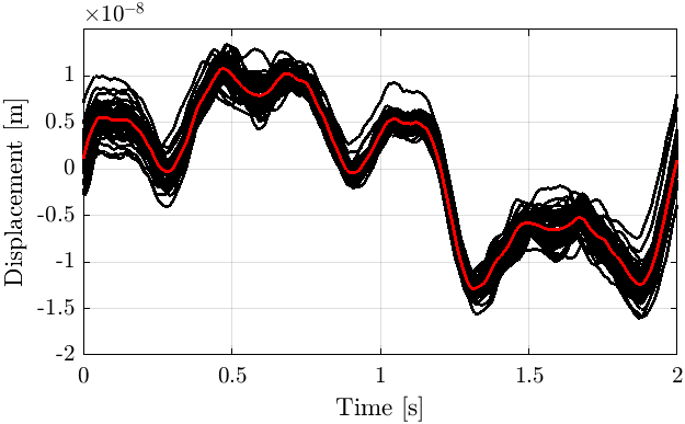
Figure 14: Difference between the two measurement in the time domain, averaged for all the cycles
3.4 Difference between Encoder and Interferometer as a function of position
Figure 14 gives the measurement error as a function of time. We here wish the compute this measurement error as a function of the position (as measured by the encoer).
To do so, all the attocube measurements corresponding to each position measured by the Encoder (resolution of \(1nm\)) are averaged. Figure 15 is obtained where we clearly see an error with a period comparable to the motion range and a much smaller period corresponding to the non-linear period errors that we wish the estimate.
  [e_sorted, ~, e_ind] = unique(encoder);

  i_mean = zeros(length(e_sorted), 1);
  for i = 1:length(e_sorted)
    i_mean(i) = mean(interferometer(e_ind == i));
  end

  i_mean_error = (i_mean - e_sorted);
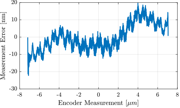
Figure 15: Difference between the two measurement as a function of the measured position by the encoder, averaged for all the cycles
The period of the non-linearity seems to be equal to \(765 nm\) which corresponds to half the wavelength of the Laser (\(1.53 \mu m\)). For the motion range done here, the non-linearity is measured over ~18 periods which permits to do some averaging.
  win_length = 1530/2; % length of the windows (corresponds to 765 nm)
  num_avg = floor(length(e_sorted)/win_length); % number of averaging

  i_init = ceil((length(e_sorted) - win_length*num_avg)/2); % does not start at the extremity

  e_sorted_mean_over_period = mean(reshape(i_mean_error(i_init:i_init+win_length*num_avg-1), [win_length num_avg]), 2);
The obtained periodic non-linearity is shown in Figure 16.
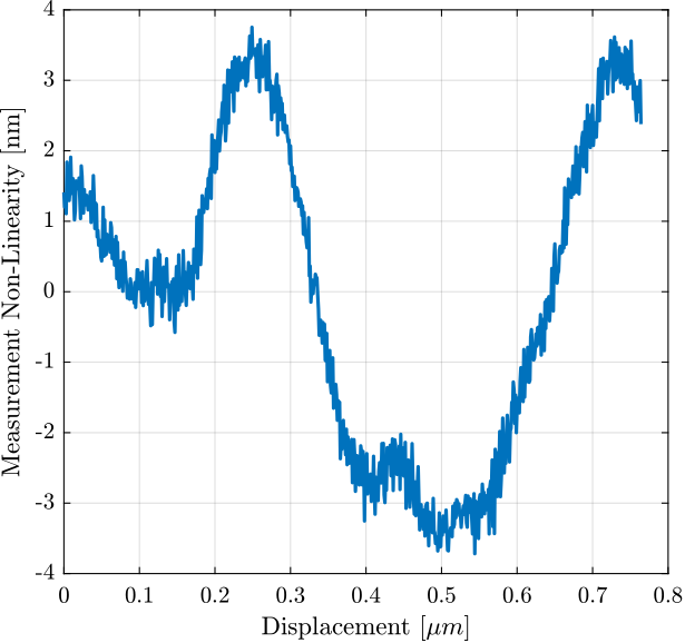
Figure 16: Non-Linearity of the Interferometer over the period of the wavelength